Let’s first check the two sftrack and sftraj objects provided in the raccoons dataset:
## sftrack (*locations*) with 445 features and 10 fields
## geometry:   "geometry" (XY, CRS: WGS 84)
## timestamps: "timestamp" (integer)
## groupings:  "sft_group" (*id*, *month*)
## -------------------------------
##   animal_id latitude longitude           timestamp height hdop vdop fix
## 1   TTP-058       NA        NA 2019-01-18 19:02:30     NA  0.0  0.0  NO
## 2   TTP-058 26.06945 -80.27906 2019-01-18 20:02:30      7  6.2  3.2  2D
## 3   TTP-058       NA        NA 2019-01-18 21:02:30     NA  0.0  0.0  NO
## 4   TTP-058       NA        NA 2019-01-18 22:02:30     NA  0.0  0.0  NO
## 5   TTP-058 26.06769 -80.27431 2019-01-18 23:02:30    858  5.1  3.2  2D
## 6   TTP-058 26.06867 -80.27930 2019-01-19 00:02:30    350  1.9  3.2  3D
##                 sft_group                   geometry
## 1 (id: TTP-058, month: 1)                POINT EMPTY
## 2 (id: TTP-058, month: 1) POINT (-80.27906 26.06945)
## 3 (id: TTP-058, month: 1)                POINT EMPTY
## 4 (id: TTP-058, month: 1)                POINT EMPTY
## 5 (id: TTP-058, month: 1) POINT (-80.27431 26.06769)
## 6 (id: TTP-058, month: 1)  POINT (-80.2793 26.06867)
racc_traj## sftraj (*steps*) with 445 features and 10 fields
## geometry: "geometry" (XY, CRS: WGS 84)
## timestamps: "timestamp" (integer)
## groupings: "sft_group" (*id*, *month*)
## -------------------------------
## animal_id latitude longitude timestamp
## 1 TTP-058 NA NA (2019-01-18 19:02:30 --> 2019-01-18 20:02:30)
## 2 TTP-058 26.06945 -80.27906 (2019-01-18 20:02:30 --> 2019-01-18 21:02:30)
## 3 TTP-058 NA NA (2019-01-18 21:02:30 --> 2019-01-18 22:02:30)
## 4 TTP-058 NA NA (2019-01-18 22:02:30 --> 2019-01-18 23:02:30)
## 5 TTP-058 26.06769 -80.27431 (2019-01-18 23:02:30 --> 2019-01-19 00:02:30)
## 6 TTP-058 26.06867 -80.27930 (2019-01-19 00:02:30 --> 2019-01-19 01:02:30)
## height hdop vdop fix sft_group geometry
## 1 NA 0.0 0.0 NO (id: TTP-058, month: 1) POINT EMPTY
## 2 7 6.2 3.2 2D (id: TTP-058, month: 1) POINT (-80.27906 26.06945)
## 3 NA 0.0 0.0 NO (id: TTP-058, month: 1) POINT EMPTY
## 4 NA 0.0 0.0 NO (id: TTP-058, month: 1) POINT EMPTY
## 5 858 5.1 3.2 2D (id: TTP-058, month: 1) LINESTRING (-80.27431 26.06...
## 6 350 1.9 3.2 3D (id: TTP-058, month: 1) LINESTRING (-80.2793 26.068...Geometry column
As stated earlier, the geometry column is built using sf, so the column functions exactly as it would in sf. You can modify it and redefine it using the sf tools. More specifically the geometry column of an sftrack object is an sfc column. The main difference between a standard sf object created using st_as_sf is that we automatically allow empty geometries, where as this option is turned off by default in st_as_sf().
racc_track$geometry## Geometry set for 445 features (with 168 geometries empty)
## Geometry type: POINT
## Dimension: XY
## Bounding box: xmin: -80.28149 ymin: 26.06761 xmax: -80.27046 ymax: 26.07706
## Geodetic CRS: WGS 84
## First 5 geometries:## POINT EMPTY## POINT (-80.27906 26.06945)## POINT EMPTY
## POINT EMPTY## POINT (-80.27431 26.06769)An sftrack object is simply an sfc of sfc_POINTS, this contrasts with an sftraj object which is a mixture of POINTs and LINESTRINGs. This is because a trajectory can have a start point and a missing end point (NA), a line segment, or a missing start point and an actual end point. As linestrings can not have NULL points in them, this allows no-loss conversion back and forth between sftrack and an sftraj.
racc_traj$geometry## Geometry set for 445 features (with 168 geometries empty)
## Geometry type: GEOMETRY
## Dimension: XY
## Bounding box: xmin: -80.28149 ymin: 26.06761 xmax: -80.27046 ymax: 26.07706
## Geodetic CRS: WGS 84
## First 5 geometries:## POINT EMPTY## POINT (-80.27906 26.06945)## POINT EMPTY
## POINT EMPTY## LINESTRING (-80.27431 26.06769, -80.2793 26.06867)This does mean that not all sf functions will handle an sftraj object like it would an sftrack if there are NAs in the data set. In these cases st_is_empty() can help to subset the points that contain geometry data.
Working with sf
As an sftrack object is an sf object, essentially all of the sf functions will work on it.
## Linking to GEOS 3.9.0, GDAL 3.2.2, PROJ 7.2.1
st_length(racc_traj)[1:10]## Units: [m]
## [1] 0.000000 0.000000 0.000000 0.000000 510.096380 107.395332
## [7] 5.625847 0.000000 0.000000 15.748173
df1 <- data.frame(
  id = c(1,1,1,1),
  time = as.POSIXct('2020-01-01 12:00:00', tz = 'UTC') + 60*60*(1:4),
  x = c(1,3,3,2),
  y = c(1,1,3,4)
)

road <- st_linestring(rbind(
  c(1,2),
  c(5,2),
  c(5,0)
)
)

animal1 <- as_sftraj(df1)
plot(animal1)
plot(road,  col = "red", add = T)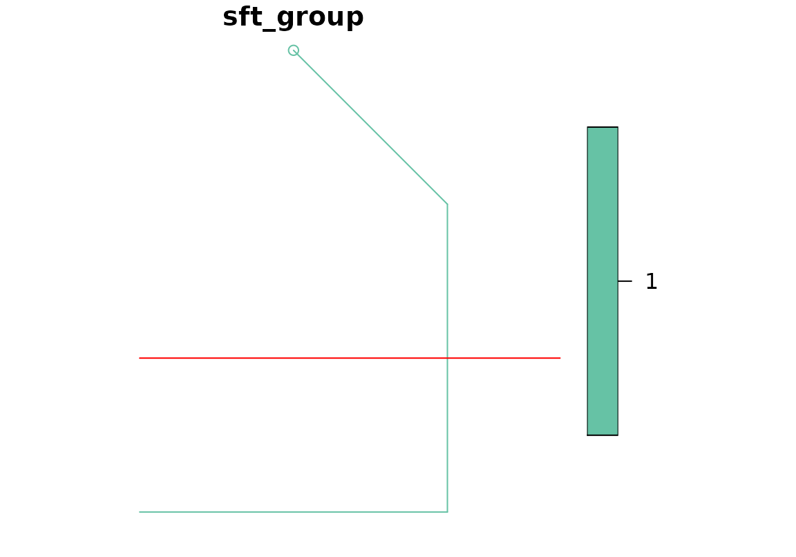
# Does the animal cross the road?
any(st_intersects(animal1, road, sparse = FALSE))
## [1] TRUE
# When?
animal1$time[st_intersects(animal1, road, sparse = FALSE)]
## [[1]]
## [1] "2020-01-01 14:00:00 UTC" "2020-01-01 15:00:00 UTC"
##
## attr(,"class")
## [1] "sft_timestamp" "list"
## attr(,"tzone")
## [1] "UTC"
## attr(,"type")
## [1] "POSIX"
# How often does the animal stay near the road?
st_is_within_distance(animal1, road, 1)
## Sparse geometry binary predicate list of length 4, where the predicate
## was `is_within_distance'
## 1: 1
## 2: 1
## 3: 1
## 4: (empty)
# How close is the animal from the road?
st_distance(animal1, road)
## [,1]
## [1,] 1
## [2,] 0
## [3,] 1
## [4,] 2The only thing to remember, is that a sftraj has a GEOMETRY column, and occasionally a function may not work with it. In those cases is_linestring() can be used to filter out incomplete steps (either missing, or without start or end point).
Plotting
Base plotting
sftrack is built to work with sf base plot methods. This means you can use most of the sf plot methods, sftrack largely just controls the grouping of the plot then feeds it back to plot.sf().
This means that everytime you change the active_group, the plot view will change.
active_group(racc_traj$sft_group) <- "id"
active_group(racc_traj$sft_group)
## [1] "id"
plot(racc_traj)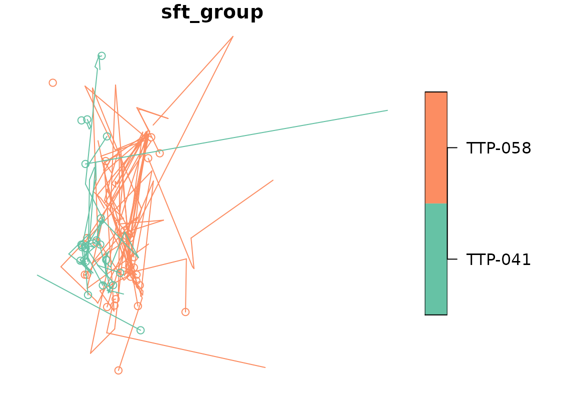
Most arguments for plot.sf are available to use as additional arguments to plot.
plot(racc_track, axes = TRUE, cex = 5)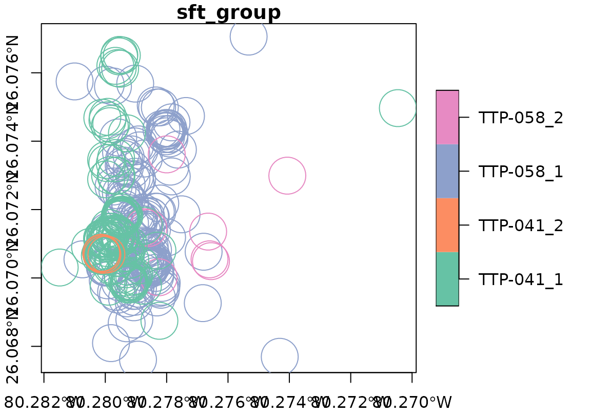
ggplot2
This is a work in progress, but theres a geom_sftrack() function that feeds geom_sf() with the correct plotting information. Like with geom_sf(), you input data into geom_sftrack() and not into ggplot(). Here too, ggplot2 assumes active_group is the grouping variable. Plots vary slightly based on if they’re sftrack of sftraj class.
geom_sftrack() is essentially geom_sf(data = data, aes(color = group_labels(data))) with NULL points subetted out. This may help when a user requires more advanced modification than the geom_sftrack() allows.
library("ggplot2")
ggplot() + geom_sftrack(data = racc_traj)
You can use geom_sftrack() just like any other ggplot2 layer, which means you can continue to make manuscript quality plots.
cols <- c("TTP-041_1" = "dodgerblue1", "TTP-041_2" = "darkseagreen2",
          "TTP-058_1" = "darkorchid1", "TTP-058_2" = "khaki3")
ggplot() +
  geom_sftrack(data = racc_track, size = 3, alpha = 0.5) +
  scale_color_manual(values = cols) +
  ggtitle("Raccoons at Tree Tops Park, Winter 2020") +
  theme_bw() +
  theme(axis.text.x = element_text(angle = 45, hjust = 1))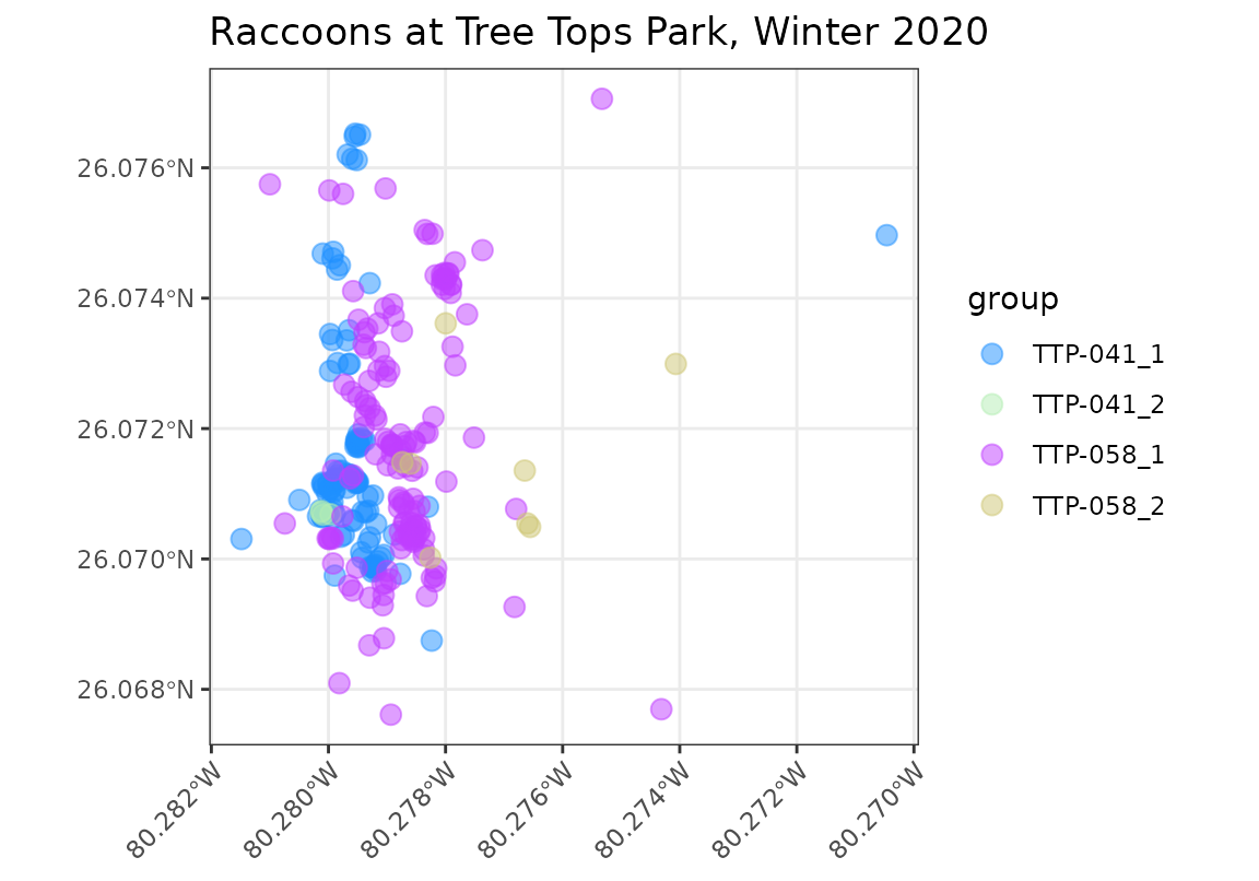
Special functions for working with an sftraj
To help with working with more complex sftraj objects, there is a growing suite of sftraj specific functions:
Step mode in plotting
sftraj objects create linestrings for each row of data, as each row is not assumed to be related to the next row of data. This data structure may become inefficient to work with when plotting large data sets. When appropriate these trajectories can be generalized by combining linestrings where lines meet.
For plotting purposes we can create these linestrings quickly and plot them at much faster speeds than individual lines.
For plot and geom_sftrack there is an argument called step_mode that refers to whether you want to plot the lines individually (step_mode = TRUE), or generalize them into connected linestrings (step_mode = FALSE). By default step_mode is set to TRUE for small datasets (less than 10,000 records), and switches to FALSE for larger datasets to enhance performance.
library("ggplot2")
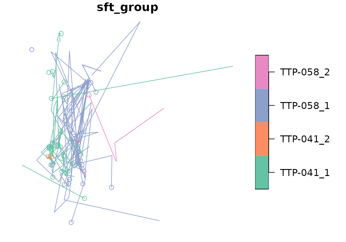
ggplot() + geom_sftrack(data = racc_traj, step_mode = TRUE) +
ggtitle("Step mode enabled")
ggplot() + geom_sftrack(data = racc_traj, step_mode = FALSE) +
ggtitle("Step mode disabled")

You’ll notice that the appearance of the plot changes as the POINTs are also displayed. This is because step mode adds POINTS to the plot that contain a fill as well as a color property.
coord_traj
This function returns a data.frame (x,y,z) of the point at \(t_1\) of each sftraj geometry. It works nearly identically to sf::st_coordinates().
coord_traj(racc_traj$geometry)[1:10, ]## [,1] [,2]
## [1,] NA NA
## [2,] -80.27906 26.06945
## [3,] NA NA
## [4,] NA NA
## [5,] -80.27431 26.06769
## [6,] -80.27930 26.06867
## [7,] -80.27908 26.06962
## [8,] -80.27902 26.06963
## [9,] NA NA
## [10,] -80.27900 26.06982
pts_traj
If youd like to retain the geometries but still pull out \(t_1\) point you can use pts_traj(). This functions returns a list of the beginning point of each sftraj geometry, or an sfc column when using the argument sfc = TRUE.
pts_traj(racc_traj$geometry)[1:5]## [[1]]## POINT EMPTY##
## [[2]]## POINT (-80.27906 26.06945)##
## [[3]]## POINT EMPTY##
## [[4]]## POINT EMPTY##
## [[5]]## POINT (-80.27431 26.06769)
pts_traj(racc_traj$geometry, sfc = TRUE)[1:5]## Geometry set for 5 features (with 3 geometries empty)
## Geometry type: POINT
## Dimension: XY
## Bounding box: xmin: -80.27906 ymin: 26.06769 xmax: -80.27431 ymax: 26.06945
## Geodetic CRS: WGS 84## POINT EMPTY## POINT (-80.27906 26.06945)## POINT EMPTY
## POINT EMPTY## POINT (-80.27431 26.06769)
is_linestring
This function may help if you’d like to quickly filter an sftraj object to just contain pure linestrings. is_linestring() returns TRUE or FALSE if the geometry is a linestring. This does not recalculate anything, it just filters out steps that contained NAs in either phase. Its nearly identical to st_is(x, "LINESTRING"), but may be more intuitive for users.
is_linestring(racc_traj$geometry)[1:10]## [1] FALSE FALSE FALSE FALSE TRUE TRUE TRUE FALSE FALSE TRUE
(new_sftraj <- racc_traj[is_linestring(racc_traj$geometry), ])## sftraj (*steps*) with 227 features and 10 fields
## geometry: "geometry" (XY, CRS: WGS 84)
## timestamps: "timestamp" (integer)
## groupings: "sft_group" (*id*)
## -------------------------------
## animal_id latitude longitude timestamp
## 5 TTP-058 26.06769 -80.27431 (2019-01-18 23:02:30 --> 2019-01-19 00:02:30)
## 6 TTP-058 26.06867 -80.27930 (2019-01-19 00:02:30 --> 2019-01-19 01:02:30)
## 7 TTP-058 26.06962 -80.27908 (2019-01-19 01:02:30 --> 2019-01-19 02:02:04)
## 10 TTP-058 26.06982 -80.27900 (2019-01-19 12:02:30 --> 2019-01-19 13:02:05)
## 11 TTP-058 26.06969 -80.27894 (2019-01-19 13:02:05 --> 2019-01-19 14:02:04)
## 12 TTP-058 26.07174 -80.27890 (2019-01-19 14:02:04 --> 2019-01-19 15:02:12)
## height hdop vdop fix sft_group geometry
## 5 858 5.1 3.2 2D (id: TTP-058, month: 1) LINESTRING (-80.27431 26.06...
## 6 350 1.9 3.2 3D (id: TTP-058, month: 1) LINESTRING (-80.2793 26.068...
## 7 11 2.3 4.5 3D (id: TTP-058, month: 1) LINESTRING (-80.27908 26.06...
## 10 NA 2.0 3.3 3D (id: TTP-058, month: 1) LINESTRING (-80.279 26.0698...
## 11 8 4.2 2.5 3D (id: TTP-058, month: 1) LINESTRING (-80.27894 26.06...
## 12 -3 0.9 1.5 3D (id: TTP-058, month: 1) LINESTRING (-80.2789 26.071...
Calculating step metrics of an sftraj
For use in movement models, you may need to calculate the \(dx\), \(dy\), length, and turn angles of each step. You can do that in sftrack using step_metrics(). It should be noted it will accept an sftrack object, however, it first converts the geometries internally to sftraj geometries and then calculates step metrics. As with other sf objects, the outcome is assumed to be in the units of the crs when not specified. Absolute angle is measured in radians.
step_metrics(racc_traj[1:10,])## dx dy dist dt abs_angle rel_angle speed
## 1 NA NA NA 3600 NA NA NA
## 2 0.000000 0.0000000 NA 3600 NA NA NA
## 3 NA NA NA 3600 NA NA NA
## 4 NA NA NA 3600 NA NA NA
## 5 498.309348 109.0329742 510.096380 3600 2.9272914 NA 0.141693439
## 6 22.473674 105.0175956 107.395332 3600 1.3588662 -1.568425 0.029832037
## 7 5.549011 0.9266259 5.625847 3574 0.1645841 -1.194282 0.001574104
## 8 0.000000 0.0000000 NA 3626 NA NA NA
## 9 NA NA NA 32400 NA NA NA
## 10 NA NA NA NA NA NA NA
## sftrack_id
## 1 TTP-058_2019-01-18 19:02:30
## 2 TTP-058_2019-01-18 20:02:30
## 3 TTP-058_2019-01-18 21:02:30
## 4 TTP-058_2019-01-18 22:02:30
## 5 TTP-058_2019-01-18 23:02:30
## 6 TTP-058_2019-01-19 00:02:30
## 7 TTP-058_2019-01-19 01:02:30
## 8 TTP-058_2019-01-19 02:02:04
## 9 TTP-058_2019-01-19 03:02:30
## 10 TTP-058_2019-01-19 12:02:30