3. Structure of sftrack/sftraj objects
Source:vignettes/sftrack3_workingwith.Rmd
sftrack3_workingwith.RmdThis is section will go more depth into the structure of sftrack/sftraj objects and how to work with them.
To begin, sftrack and sftraj objects are essentially data.frame objects with the 3 required columns (group, geometry, and time). However, they are also of the subclass sf. This allows them to act like sf objects when working with functions in the sf package but act as sftrack objects for all other actions. It should be noted that when possible sftrack objects will mimic sf functionality and thus many of the same words and tactics are used.
## sftrack (*locations*) with 445 features and 10 fields
## geometry:   "geometry" (XY, CRS: WGS 84)
## timestamps: "timestamp" (integer)
## groupings:  "sft_group" (*id*, *month*)
## -------------------------------
##   animal_id latitude longitude           timestamp height hdop vdop fix
## 1   TTP-058       NA        NA 2019-01-18 19:02:30     NA  0.0  0.0  NO
## 2   TTP-058 26.06945 -80.27906 2019-01-18 20:02:30      7  6.2  3.2  2D
## 3   TTP-058       NA        NA 2019-01-18 21:02:30     NA  0.0  0.0  NO
## 4   TTP-058       NA        NA 2019-01-18 22:02:30     NA  0.0  0.0  NO
## 5   TTP-058 26.06769 -80.27431 2019-01-18 23:02:30    858  5.1  3.2  2D
## 6   TTP-058 26.06867 -80.27930 2019-01-19 00:02:30    350  1.9  3.2  3D
##                 sft_group                   geometry
## 1 (id: TTP-058, month: 1)                POINT EMPTY
## 2 (id: TTP-058, month: 1) POINT (-80.27906 26.06945)
## 3 (id: TTP-058, month: 1)                POINT EMPTY
## 4 (id: TTP-058, month: 1)                POINT EMPTY
## 5 (id: TTP-058, month: 1) POINT (-80.27431 26.06769)
## 6 (id: TTP-058, month: 1)  POINT (-80.2793 26.06867)
racc_traj## sftraj (*steps*) with 445 features and 10 fields
## geometry: "geometry" (XY, CRS: WGS 84)
## timestamps: "timestamp" (integer)
## groupings: "sft_group" (*id*, *month*)
## -------------------------------
## animal_id latitude longitude timestamp
## 1 TTP-058 NA NA (2019-01-18 19:02:30 --> 2019-01-18 20:02:30)
## 2 TTP-058 26.06945 -80.27906 (2019-01-18 20:02:30 --> 2019-01-18 21:02:30)
## 3 TTP-058 NA NA (2019-01-18 21:02:30 --> 2019-01-18 22:02:30)
## 4 TTP-058 NA NA (2019-01-18 22:02:30 --> 2019-01-18 23:02:30)
## 5 TTP-058 26.06769 -80.27431 (2019-01-18 23:02:30 --> 2019-01-19 00:02:30)
## 6 TTP-058 26.06867 -80.27930 (2019-01-19 00:02:30 --> 2019-01-19 01:02:30)
## height hdop vdop fix sft_group geometry
## 1 NA 0.0 0.0 NO (id: TTP-058, month: 1) POINT EMPTY
## 2 7 6.2 3.2 2D (id: TTP-058, month: 1) POINT (-80.27906 26.06945)
## 3 NA 0.0 0.0 NO (id: TTP-058, month: 1) POINT EMPTY
## 4 NA 0.0 0.0 NO (id: TTP-058, month: 1) POINT EMPTY
## 5 858 5.1 3.2 2D (id: TTP-058, month: 1) LINESTRING (-80.27431 26.06...
## 6 350 1.9 3.2 3D (id: TTP-058, month: 1) LINESTRING (-80.2793 26.068...In order for sftrack to function as an sf object, we create the data object as an sf object first (using st_as_sf()), and then add the sftrack attributes to the object. The class of an sftrack object is sftrack -> sf -> data.frame although the data.frame class is rarely called upon.
class(racc_track)## [1] "sftrack" "sf" "data.frame"There are five attributes total to an sftrack object, two of these are created by sf (sf_column and agr), and the additional three are created by sftrack (group_col, time_col, and error_col).
attributes(racc_track)[-(1:2)]## $class
## [1] "sftrack" "sf" "data.frame"
##
## $sf_column
## [1] "geometry"
##
## $agr
## animal_id latitude longitude timestamp height hdop vdop fix
## <NA> <NA> <NA> <NA> <NA> <NA> <NA> <NA>
## sft_group
## <NA>
## Levels: constant aggregate identity
##
## $group_col
## [1] "sft_group"
##
## $time_col
## [1] "timestamp"
##
## $error_col
## [1] NAThe sftrack level attributes are simply pointers to the data. Any attributes relevant to the grouping or geometry are stored in those columns themselves.
Geometry
The geometry column is an sfc object and contains the important spatial information for the track. As NA points are common and important in movement data, we create the sfc object with the argument na.fail = FALSE.
racc_track$geometry## Geometry set for 445 features (with 168 geometries empty)
## Geometry type: POINT
## Dimension: XY
## Bounding box: xmin: -80.28149 ymin: 26.06761 xmax: -80.27046 ymax: 26.07706
## Geodetic CRS: WGS 84
## First 5 geometries:## POINT EMPTY## POINT (-80.27906 26.06945)## POINT EMPTY
## POINT EMPTY## POINT (-80.27431 26.06769)The sfc column varies in structure dependent on the movement class. An sftrack is a collection of POINTs while an sftraj is a GEOMETRY collection of POINTs and LINESTRINGs.
df1 <- data.frame(
  id = c(1, 1, 1, 1, 1, 1),
  month = c(1, 1, 1, 1, 1, 1),
  x = c(27, 27, 27, NA, 29, 30),
  y = c(-80, -81, -82, NA, 83, 83),
  timez = as.POSIXct("2020-01-01 12:00:00", tz = "UTC") + 60*60*(1:6)
)

test_sftraj <- as_sftraj(data = df1, group = list(id = df1$id, month = df1$month),
                         time = df1$timez, active_group = c("id","month"),
                         coords = df1[, c("x", "y")])
test_sftraj$geometry
## Geometry set for 6 features (with 1 geometry empty)
## Geometry type: GEOMETRY
## Dimension: XY
## Bounding box: xmin: 27 ymin: -82 xmax: 30 ymax: 83
## CRS: NA
## First 5 geometries:## LINESTRING (27 -80, 27 -81)## LINESTRING (27 -81, 27 -82)## POINT (27 -82)## POINT EMPTY## LINESTRING (29 83, 30 83)Grouping
The grouping column is very specialized, and we will cover it in its own section. To begin, the novel attributes it stores are the active_group and the sort_index which is a factor of the current active groups. The grouping class consists of single row level group: s_groups (a.k.a single groups) and a column level collection of s_groups called a c_grouping (a.k.a column/collection grouping). This column acts as a robust storage column for the groupings and is maintained across a sftrack object.
attributes(racc_track$sft_group[1:10])## $active_group
## [1] "id" "month"
##
## $sort_index
## [1] TTP-058_1 TTP-058_1 TTP-058_1 TTP-058_1 TTP-058_1 TTP-058_1 TTP-058_1
## [8] TTP-058_1 TTP-058_1 TTP-058_1
## Levels: TTP-058_1
##
## $class
## [1] "c_grouping"
summary(racc_track)## animal_id latitude longitude timestamp
## TTP-041:223 Min. :26.07 Min. :-80.28 Min. :2019-01-18 19:02:30
## TTP-058:222 1st Qu.:26.07 1st Qu.:-80.28 1st Qu.:2019-01-22 02:02:30
## Median :26.07 Median :-80.28 Median :2019-01-25 18:02:30
## Mean :26.07 Mean :-80.28 Mean :2019-01-25 17:22:18
## 3rd Qu.:26.07 3rd Qu.:-80.28 3rd Qu.:2019-01-29 02:02:09
## Max. :26.08 Max. :-80.27 Max. :2019-02-01 18:02:30
## NA's :168 NA's :168
## height hdop vdop fix
## Min. : -30.00 Min. :0.000 Min. :0.000 2D: 37
## 1st Qu.: 1.00 1st Qu.:0.000 1st Qu.:0.000 3D:240
## Median : 7.00 Median :1.300 Median :1.900 NO:168
## Mean : 36.65 Mean :1.691 Mean :1.938
## 3rd Qu.: 15.50 3rd Qu.:2.500 3rd Qu.:3.200
## Max. :1107.00 Max. :9.900 Max. :8.400
## NA's :198
## sft_group geometry
## TTP-041_1 :213 POINT :445
## TTP-041_2 : 10 epsg:4326 : 0
## TTP-058_1 :212 +proj=long...: 0
## TTP-058_2 : 10
## active_group: id, month: 0
##
## Time
The time column must be either an integer or POSIXct and the column must be of one type of time. Beyond that there is not much specialized functionality in the column. Sftrack uses the time column to order outputs for analysis, and attempts to order outputs when originally making an sftrack object, however, the data.frame is not required to be ordered for analysis. A call to check_ordered() is called before analysis, and otherwise it is assumed the order does not matter. This is particularly true for a sftraj, where the geometry level contains information about t1 and t2.
Error
The error column is the column with the relevant error information for the spatial points in it. At present we have not built particular functionality but plan to in the future or reserve this for other developers to build upon.
Subsetting
An sftrack object acts like a data.frame and sf whenever appropriate. Because of this you can subset an sftrack object as you would a data.frame.
In this way row subsetting is very straight forward, as each row represents an individual point in time.
racc_track[1:10, ]## sftrack (*locations*) with 10 features and 10 fields
## geometry: "geometry" (XY, CRS: WGS 84)
## timestamps: "timestamp" (integer)
## groupings: "sft_group" (*id*, *month*)
## -------------------------------
## animal_id latitude longitude timestamp height hdop vdop fix
## 1 TTP-058 NA NA 2019-01-18 19:02:30 NA 0.0 0.0 NO
## 2 TTP-058 26.06945 -80.27906 2019-01-18 20:02:30 7 6.2 3.2 2D
## 3 TTP-058 NA NA 2019-01-18 21:02:30 NA 0.0 0.0 NO
## 4 TTP-058 NA NA 2019-01-18 22:02:30 NA 0.0 0.0 NO
## 5 TTP-058 26.06769 -80.27431 2019-01-18 23:02:30 858 5.1 3.2 2D
## 6 TTP-058 26.06867 -80.27930 2019-01-19 00:02:30 350 1.9 3.2 3D
## sft_group geometry
## 1 (id: TTP-058, month: 1) POINT EMPTY
## 2 (id: TTP-058, month: 1) POINT (-80.27906 26.06945)
## 3 (id: TTP-058, month: 1) POINT EMPTY
## 4 (id: TTP-058, month: 1) POINT EMPTY
## 5 (id: TTP-058, month: 1) POINT (-80.27431 26.06769)
## 6 (id: TTP-058, month: 1) POINT (-80.2793 26.06867)Unlike a data.frame, however, sftrack attempts to retain the geometry, group, and time columns, in order to maintain sftrack status. This is similar to how sf deals with the geometry column.
racc_track[1:3, c(1:3)]## sftrack (*locations*) with 3 features and 6 fields
## geometry: "geometry" (XY, CRS: WGS 84)
## timestamps: "timestamp" (integer)
## groupings: "sft_group" (*id*, *month*)
## -------------------------------
## animal_id latitude longitude sft_group timestamp
## 1 TTP-058 NA NA (id: TTP-058, month: 1) 2019-01-18 19:02:30
## 2 TTP-058 26.06945 -80.27906 (id: TTP-058, month: 1) 2019-01-18 20:02:30
## 3 TTP-058 NA NA (id: TTP-058, month: 1) 2019-01-18 21:02:30
## geometry
## 1 POINT EMPTY
## 2 POINT (-80.27906 26.06945)
## 3 POINT EMPTYTo turn off this feature, you use the drop = T argument which returns a data.frame object instead. If youd like to revert to an sf object, sf::st_sf(data) will return the object to an sf object.
racc_track[1:3, c(1:3), drop = TRUE]## animal_id latitude longitude
## 1 TTP-058 NA NA
## 2 TTP-058 26.06945 -80.27906
## 3 TTP-058 NA NAsftrajs work nearly the same as sftracks, however because they are a step model where the steps are modeled as step1 (\(t_1 → t_2\)) its important to note that subsetting will not automatically recalculate any new steps for you even if the original \(t_2\) point has been deleted.
If your subsetting will also change the end points for steps, then you can recalculate using step_recalc(). The output which is your original sftraj object but with the geometry column recalculated to the new t2s based on the timestamp. The results of which can be wildly different than the original subsetted data.frame. So be careful.
plot(racc_traj, main = "Original")
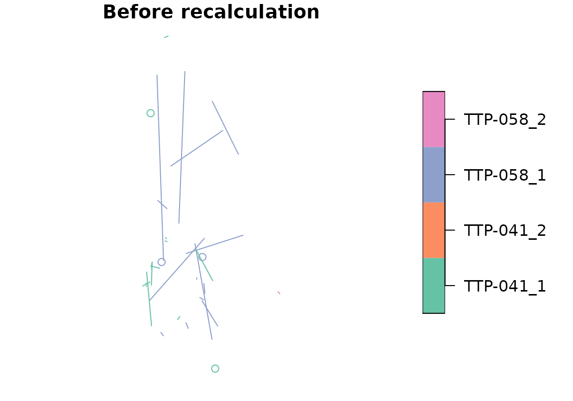
plot(step_recalc(new_traj), main = "After recalculation")
Some basic methods and functions of sftrack and sftraj objects
print
The print() layout is a modified version of the sf print function. It returns important info summarizing the sftrack object like the geometry information and grouping information. The print function defaults to printing 6 rows and displaying all the columns. This can be modified using the n and n_col arguments, which subset the printed output in the respective dimensions (use n = Inf to print all rows). When using n_col the display will show the grouping geometry, and time fields as well as any other columns starting from column 1 until #columns + 3 = n_col. n and n_col are optional arguments, and if values are not supplied they default to the data.frame defaults. Note: n is not a corrolary to head(), as head() physically subsets the data while the n option just modifies the printed output.
print(racc_track, 5, 10)## sftrack (*locations*) with 445 features and 10 fields
## geometry: "geometry" (XY, CRS: WGS 84)
## timestamps: "timestamp" (integer)
## groupings: "sft_group" (*id*, *month*)
## -------------------------------
## animal_id latitude longitude timestamp height hdop vdop fix
## 1 TTP-058 NA NA 2019-01-18 19:02:30 NA 0.0 0.0 NO
## 2 TTP-058 26.06945 -80.27906 2019-01-18 20:02:30 7 6.2 3.2 2D
## 3 TTP-058 NA NA 2019-01-18 21:02:30 NA 0.0 0.0 NO
## 4 TTP-058 NA NA 2019-01-18 22:02:30 NA 0.0 0.0 NO
## 5 TTP-058 26.06769 -80.27431 2019-01-18 23:02:30 858 5.1 3.2 2D
## sft_group geometry
## 1 (id: TTP-058, month: 1) POINT EMPTY
## 2 (id: TTP-058, month: 1) POINT (-80.27906 26.06945)
## 3 (id: TTP-058, month: 1) POINT EMPTY
## 4 (id: TTP-058, month: 1) POINT EMPTY
## 5 (id: TTP-058, month: 1) POINT (-80.27431 26.06769)
summary
summary() works as youd expect for a data.frame, except it displays the grouping column as a count of each active_group combination and the active_groupfor that column.
summary(racc_track)## animal_id latitude longitude timestamp
## TTP-041:223 Min. :26.07 Min. :-80.28 Min. :2019-01-18 19:02:30
## TTP-058:222 1st Qu.:26.07 1st Qu.:-80.28 1st Qu.:2019-01-22 02:02:30
## Median :26.07 Median :-80.28 Median :2019-01-25 18:02:30
## Mean :26.07 Mean :-80.28 Mean :2019-01-25 17:22:18
## 3rd Qu.:26.07 3rd Qu.:-80.28 3rd Qu.:2019-01-29 02:02:09
## Max. :26.08 Max. :-80.27 Max. :2019-02-01 18:02:30
## NA's :168 NA's :168
## height hdop vdop fix
## Min. : -30.00 Min. :0.000 Min. :0.000 2D: 37
## 1st Qu.: 1.00 1st Qu.:0.000 1st Qu.:0.000 3D:240
## Median : 7.00 Median :1.300 Median :1.900 NO:168
## Mean : 36.65 Mean :1.691 Mean :1.938
## 3rd Qu.: 15.50 3rd Qu.:2.500 3rd Qu.:3.200
## Max. :1107.00 Max. :9.900 Max. :8.400
## NA's :198
## sft_group geometry
## TTP-041_1 :213 POINT :445
## TTP-041_2 : 10 epsg:4326 : 0
## TTP-058_1 :212 +proj=long...: 0
## TTP-058_2 : 10
## active_group: id, month: 0
##
##
group_summary
group_summary() is a special summary function specific for sftrack and sftraj objects. It summarizes the data based on the beginning and end of each grouping as well as the total distance and area covered by the grouping. This function uses st_distance andst_convex_hull from the sf package and therefore outputs in units of the CRS. In this example the distance is in meters.
group_summary(racc_track)## group n_records NAs begin_time end_time length.m
## 1 TTP-041_1 213 95 2019-01-18 19:02:30 2019-01-31 23:02:30 10125.58779
## 2 TTP-041_2 10 6 2019-02-01 00:02:30 2019-02-01 18:02:07 32.28359
## 3 TTP-058_1 212 65 2019-01-18 19:02:30 2019-01-31 23:02:11 25213.34945
## 4 TTP-058_2 10 2 2019-02-01 00:02:05 2019-02-01 18:02:30 1499.89984
## area.m.2
## 1 510731.47739
## 2 50.13265
## 3 569641.54591
## 4 108199.81171You can also trigger this function by using summary(<data>, by_group = TRUE)
summary(racc_track, by_group = TRUE)## group n_records NAs begin_time end_time length.m
## 1 TTP-041_1 213 95 2019-01-18 19:02:30 2019-01-31 23:02:30 10125.58779
## 2 TTP-041_2 10 6 2019-02-01 00:02:30 2019-02-01 18:02:07 32.28359
## 3 TTP-058_1 212 65 2019-01-18 19:02:30 2019-01-31 23:02:11 25213.34945
## 4 TTP-058_2 10 2 2019-02-01 00:02:05 2019-02-01 18:02:30 1499.89984
## area.m.2
## 1 510731.47739
## 2 50.13265
## 3 569641.54591
## 4 108199.81171