We now have a problem, a team, and use cases to consider for our sftraj package. In order to be relevant, we also need to know what does already exist in R, what other projects have attempted to deal with trajectories and tracking data, and what lessons can we learn from this. In this post of the sftraj series, we thus review the state of affairs in the R world. Several packages have attempted to define classes for trajectories. They notably include, chronologically, adehabitatLT, trip, move, trajectories, trackerR and amt.
Table of Contents
- Class
ltraj(packageadehabitatLT) - Class
trip(packagetrip) - Classes
MoveandMoveStack(packagemove) - Classes
Track,TracksandTracksCollection(packagetrajectories) - Class
trackeRdata(packagetrackeR) - Classes
track_xyandtrack_xyt(packageamt) - Concluding remarks
We will present the classes of each of them, using movement data from fishers (Martes pennanti) tracked near Albany, New York, USA, which is stored as example data in the package move:
fisher_data <- read.table(system.file("extdata", "fishersSubset.csv.gz", package = "move"), header = TRUE, sep = ",", dec = ".")
fisher_data <- fisher_data[, c("timestamp", "ground.speed", "heading", "utm.easting", "utm.northing", "utm.zone", "location.long", "location.lat", "sensor", "individual.local.identifier", "study.name", "study.timezone")]
fisher_data$timestamp <- as.POSIXct(fisher_data$timestamp, format = "%Y-%m-%d %H:%M:%S", tz = "UTC")
head(fisher_data)
## timestamp ground.speed heading utm.easting utm.northing
## 1 2009-02-11 12:16:45 2.10 125.17 590130.0 4732942
## 2 2009-02-11 12:31:38 0.51 3.28 590136.3 4732940
## 3 2009-02-11 12:45:48 0.16 91.10 590138.5 4732935
## 4 2009-02-11 13:00:16 0.23 335.54 590144.0 4732947
## 5 2009-02-11 13:15:19 0.48 359.79 590137.0 4732940
## 6 2009-02-11 13:30:13 0.17 29.49 590126.0 4732936
## utm.zone location.long location.lat sensor individual.local.identifier
## 1 18N -73.89880 42.74370 gps Leroy
## 2 18N -73.89872 42.74369 gps Leroy
## 3 18N -73.89869 42.74364 gps Leroy
## 4 18N -73.89862 42.74374 gps Leroy
## 5 18N -73.89871 42.74368 gps Leroy
## 6 18N -73.89885 42.74365 gps Leroy
## study.name study.timezone
## 1 Urban fisher GPS tracking Eastern Standard Time
## 2 Urban fisher GPS tracking Eastern Standard Time
## 3 Urban fisher GPS tracking Eastern Standard Time
## 4 Urban fisher GPS tracking Eastern Standard Time
## 5 Urban fisher GPS tracking Eastern Standard Time
## 6 Urban fisher GPS tracking Eastern Standard TimeThis dataset contains tracking data for two individuals (Leroy and Ricky.T), with coordinates available as longitude/latitude, but also projected in UTM 18N. We convert the timestamps to a true POSIXct time in R, with the UTC timezone.
Class ltraj (package adehabitatLT)
Developed as early as 2006 (back then in the ancestor package adehabitat), the class ltraj was the first class dedicated to movement that relied on a conceptual data model, based on the idea of successive steps, i.e. the straight-line segment connecting two successive locations (Calenge et al. 20091).
Several descriptive parameters of the trajectory are automatically computed in a object of class ltraj (Figure below): parameters describing each step (increments in the X and Y directions, respectively \(\delta x\) and \(\delta y\), the step length \(d\) and the absolute angle between the step and the X direction \(α\)) (A); the relative angle \(ρ\) (B), which measures the angle between the current step and the direction of the previous step; the mean squared displacement \(R_n^2\), which is the square of the distance between the first relocation and the current relocation of the animal (C).
 Descriptive parameters of a trajectory.
We can create a ltraj object with as.ltraj, which basically expects a set of coordinates (in a data.frame), and vectors of associated timestamps and individual identification. Additional data can be provided in infolocs, and the actual projection of the data in proj4string. Because of the geometrical model, adehabitatLT expects projected coordinates. We thus use directly the UTM coordinates:
library("adehabitatLT")
(fisher_ltraj <- adehabitatLT::as.ltraj(xy = fisher_data[, c("utm.easting", "utm.northing")],
    date = fisher_data$timestamp,
    id = fisher_data$individual.local.identifier,
    infolocs = fisher_data[, !(names(fisher_data) %in% c("timestamp", "utm.easting", "utm.northing", "individual.local.identifier"))],
    proj4string = CRS("+proj=utm +zone=18 +ellps=WGS84 +datum=WGS84 +units=m +no_defs")))
##
## *********** List of class ltraj ***********
##
## Type of the traject: Type II (time recorded)
## * Time zone: UTC *
## Irregular traject. Variable time lag between two locs
##
## Characteristics of the bursts:
## id burst nb.reloc NAs date.begin date.end
## 1 Leroy Leroy 500 0 2009-02-11 12:16:45 2009-02-23 06:30:29
## 2 Ricky.T Ricky.T 700 0 2010-02-09 17:01:23 2010-02-16 04:28:08
##
##
## infolocs provided. The following variables are available:
## [1] "ground.speed" "heading" "utm.zone" "location.long"
## [5] "location.lat" "sensor" "study.name" "study.timezone"plot(fisher_ltraj)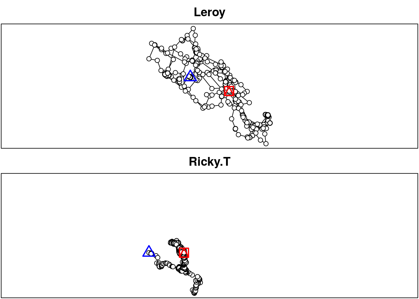
Printing the object shows an informative summary providing general information about the data (is the time recorded?, time zone, is the trajectory regular in time?) and characteristics of individual bursts. In adehabitatLT, a burst is an elementary sequence of steps, so each individual can have several bursts (e.g. associated to different GPS collars or different routes). Information associated to each burst in the summary shows the individual ID, the burst, the total number of locations (i.e. number of records), the number of missing locations, and the start and end date of the monitoring. Note that additional data is provided as infolocs (more on that below).
General information about the data is stored as global attributes of the object. The ltraj class relies on an ad-hoc list structure, where each element is a burst, stored as a data.frame:
attributes(fisher_ltraj)## $class
## [1] "ltraj" "list"
##
## $typeII
## [1] TRUE
##
## $regular
## [1] FALSE
##
## $proj4string
## CRS arguments:
## +proj=utm +zone=18 +ellps=WGS84 +datum=WGS84 +units=m +no_defs
## +towgs84=0,0,0class(fisher_ltraj)## [1] "ltraj" "list"length(fisher_ltraj)## [1] 2head(fisher_ltraj[[1]])## x y date dx dy dist dt
## 1 590130.0 4732942 2009-02-11 12:16:45 6.269668 -1.184329 6.380546 893
## 2 590136.3 4732940 2009-02-11 12:31:38 2.220108 -5.146609 5.605039 850
## 3 590138.5 4732935 2009-02-11 12:45:48 5.499546 11.411379 12.667461 868
## 4 590144.0 4732947 2009-02-11 13:00:16 -6.944491 -6.698911 9.648905 903
## 5 590137.0 4732940 2009-02-11 13:15:19 -11.083026 -3.843022 11.730400 894
## 6 590126.0 4732936 2009-02-11 13:30:13 13.220912 4.370704 13.924639 924
## R2n abs.angle rel.angle
## 1 0.00000 -0.1866983 NA
## 2 40.71137 -1.1635402 -0.9768419
## 3 112.15707 1.1217047 2.2852449
## 4 221.51200 -2.3741925 2.7872882
## 5 52.24908 -2.8078175 -0.4336250
## 6 46.13493 0.3192797 3.1270972Modifying an object means manipulating the elements of the list. For instance, manually changing the X coordinate of a location to NA requires accessing the burst's data.frame (here we modify the 4th record of the first burst):
fisher_ltraj[[1]][4, "x"] <- NA
head(fisher_ltraj[[1]])
## x y date dx dy dist dt
## 1 590130.0 4732942 2009-02-11 12:16:45 6.269668 -1.184329 6.380546 893
## 2 590136.3 4732940 2009-02-11 12:31:38 2.220108 -5.146609 5.605039 850
## 3 590138.5 4732935 2009-02-11 12:45:48 5.499546 11.411379 12.667461 868
## 4 NA 4732947 2009-02-11 13:00:16 -6.944491 -6.698911 9.648905 903
## 5 590137.0 4732940 2009-02-11 13:15:19 -11.083026 -3.843022 11.730400 894
## 6 590126.0 4732936 2009-02-11 13:30:13 13.220912 4.370704 13.924639 924
## R2n abs.angle rel.angle
## 1 0.00000 -0.1866983 NA
## 2 40.71137 -1.1635402 -0.9768419
## 3 112.15707 1.1217047 2.2852449
## 4 221.51200 -2.3741925 2.7872882
## 5 52.24908 -2.8078175 -0.4336250
## 6 46.13493 0.3192797 3.1270972As we can see above, the descriptive parameters are now out of sync. adehabitatLT thus offers a function rec, which simply recompute all descriptive parameters:
fisher_ltraj <- adehabitatLT::rec(fisher_ltraj)
head(fisher_ltraj[[1]])
## x y date dx dy dist dt
## 1 590130.0 4732942 2009-02-11 12:16:45 6.269668 -1.184329 6.380546 893
## 2 590136.3 4732940 2009-02-11 12:31:38 2.220108 -5.146609 5.605039 850
## 3 590138.5 4732935 2009-02-11 12:45:48 NA 11.411379 NA 868
## 4 NA 4732947 2009-02-11 13:00:16 NA -6.698911 NA 903
## 5 590137.0 4732940 2009-02-11 13:15:19 -11.083026 -3.843022 11.730400 894
## 6 590126.0 4732936 2009-02-11 13:30:13 13.220912 4.370704 13.924639 924
## R2n abs.angle rel.angle
## 1 0.00000 -0.1866983 NA
## 2 40.71137 -1.1635402 -0.9768419
## 3 112.15707 NA NA
## 4 NA NA NA
## 5 52.24908 -2.8078175 NA
## 6 46.13493 0.3192797 3.1270972Note that many functions working on ltraj actually automatically recompute descriptive parameters — which can be an issue in some cases where the change was meant to stay.
As seen above, bursts do not show the individual identification, the burst, or additional data. All are actually stored as attributes of the burst itself, with accessor functions to retrieve (or modify) them:
lapply(attributes(fisher_ltraj[[1]]), head)## $names
## [1] "x" "y" "date" "dx" "dy" "dist"
##
## $row.names
## [1] "1" "2" "3" "4" "5" "6"
##
## $class
## [1] "data.frame"
##
## $id
## [1] "Leroy"
##
## $burst
## [1] "Leroy"
##
## $infolocs
##   ground.speed heading utm.zone location.long location.lat sensor
## 1         2.10  125.17      18N     -73.89880     42.74370    gps
## 2         0.51    3.28      18N     -73.89872     42.74369    gps
## 3         0.16   91.10      18N     -73.89869     42.74364    gps
## 4         0.23  335.54      18N     -73.89862     42.74374    gps
## 5         0.48  359.79      18N     -73.89871     42.74368    gps
## 6         0.17   29.49      18N     -73.89885     42.74365    gps
##                  study.name        study.timezone
## 1 Urban fisher GPS tracking Eastern Standard Time
## 2 Urban fisher GPS tracking Eastern Standard Time
## 3 Urban fisher GPS tracking Eastern Standard Time
## 4 Urban fisher GPS tracking Eastern Standard Time
## 5 Urban fisher GPS tracking Eastern Standard Time
## 6 Urban fisher GPS tracking Eastern Standard TimeadehabitatLT::id(fisher_ltraj)## [1] "Leroy" "Ricky.T"adehabitatLT::burst(fisher_ltraj)## [1] "Leroy" "Ricky.T"class(adehabitatLT::infolocs(fisher_ltraj))## [1] "list"head(adehabitatLT::infolocs(fisher_ltraj)[[1]])## ground.speed heading utm.zone location.long location.lat sensor
## 1 2.10 125.17 18N -73.89880 42.74370 gps
## 2 0.51 3.28 18N -73.89872 42.74369 gps
## 3 0.16 91.10 18N -73.89869 42.74364 gps
## 4 0.23 335.54 18N -73.89862 42.74374 gps
## 5 0.48 359.79 18N -73.89871 42.74368 gps
## 6 0.17 29.49 18N -73.89885 42.74365 gps
## study.name study.timezone
## 1 Urban fisher GPS tracking Eastern Standard Time
## 2 Urban fisher GPS tracking Eastern Standard Time
## 3 Urban fisher GPS tracking Eastern Standard Time
## 4 Urban fisher GPS tracking Eastern Standard Time
## 5 Urban fisher GPS tracking Eastern Standard Time
## 6 Urban fisher GPS tracking Eastern Standard TimeNote that the additional information (stored in infolocs) is actually retrieve as a list, again with one element per burst.
Altogether, the use of a list makes ltraj objects rather complicated to use, requiring to frequently go back and forth between ltrajs and data.frames, for which most users are much more familiar with. adehabitatLT provides two helper functions to convert from ltraj to data.frame (ld) and vice versa (dl):
head(ld(fisher_ltraj))## x y date dx dy dist dt
## 1 590130.0 4732942 2009-02-11 12:16:45 6.269668 -1.184329 6.380546 893
## 2 590136.3 4732940 2009-02-11 12:31:38 2.220108 -5.146609 5.605039 850
## 3 590138.5 4732935 2009-02-11 12:45:48 NA 11.411379 NA 868
## 4 NA 4732947 2009-02-11 13:00:16 NA -6.698911 NA 903
## 5 590137.0 4732940 2009-02-11 13:15:19 -11.083026 -3.843022 11.730400 894
## 6 590126.0 4732936 2009-02-11 13:30:13 13.220912 4.370704 13.924639 924
## R2n abs.angle rel.angle id burst ground.speed heading
## 1 0.00000 -0.1866983 NA Leroy Leroy 2.10 125.17
## 2 40.71137 -1.1635402 -0.9768419 Leroy Leroy 0.51 3.28
## 3 112.15707 NA NA Leroy Leroy 0.16 91.10
## 4 NA NA NA Leroy Leroy 0.23 335.54
## 5 52.24908 -2.8078175 NA Leroy Leroy 0.48 359.79
## 6 46.13493 0.3192797 3.1270972 Leroy Leroy 0.17 29.49
## utm.zone location.long location.lat sensor study.name
## 1 18N -73.89880 42.74370 gps Urban fisher GPS tracking
## 2 18N -73.89872 42.74369 gps Urban fisher GPS tracking
## 3 18N -73.89869 42.74364 gps Urban fisher GPS tracking
## 4 18N -73.89862 42.74374 gps Urban fisher GPS tracking
## 5 18N -73.89871 42.74368 gps Urban fisher GPS tracking
## 6 18N -73.89885 42.74365 gps Urban fisher GPS tracking
## study.timezone
## 1 Eastern Standard Time
## 2 Eastern Standard Time
## 3 Eastern Standard Time
## 4 Eastern Standard Time
## 5 Eastern Standard Time
## 6 Eastern Standard Timedim(ld(fisher_ltraj))## [1] 1200 20Class trip (package trip)
Also developed in 2006, the package trip provides a class trip for trajectories. This is a S4 class directly extending sp’s SpatialPointsDataFrame class to connect series of points with a column of timestamps. The connection is made through a TimeOrderedRecords object that identifies which data columns corresponds to timestamps and identity of the moving object. A trip can be created either from a data.frame (which assumes that the first four columns provide x-, y-, time-coordinates, and individual ID) or directly from a SpatialPointsDataFrame (which allows to define which columns to use). To keep it simple, we convert the original data to a SpatialPointsDataFrame:
library("trip")
fisher_data_sp <- SpatialPointsDataFrame(coords = fisher_data[, c("location.long", "location.lat")],
    data = fisher_data[, !(names(fisher_data) %in% c("location.long", "location.lat"))],
    coords.nrs = numeric(0),
    proj4string = CRS("+proj=longlat +ellps=WGS84"))
(fisher_trip <- trip::trip(obj = fisher_data_sp, TORnames = c("timestamp", "individual.local.identifier")))
##
## Object of class trip
## tripID ("individual.local.identifier") No.Records
## 1 Leroy 500
## 2 Ricky.T 700
## startTime ("timestamp") endTime ("timestamp") tripDuration
## 1 2009-02-11 12:16:45 2009-02-23 06:30:29 11.75954 days
## 2 2010-02-09 17:01:23 2010-02-16 04:28:08 6.47691 days
##
## data.columns data.class
## 1 timestamp POSIXct **trip DateTime**
## 2 ground.speed numeric
## 3 heading numeric
## 4 utm.easting numeric
## 5 utm.northing numeric
## 6 utm.zone factor
## 7 sensor factor
## 8 individual.local.identifier factor **trip ID**
## 9 study.name factor
## 10 study.timezone factorplot(fisher_trip)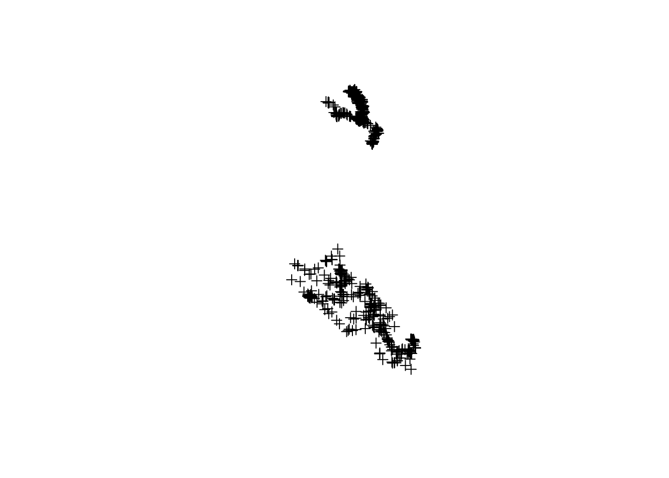
Printing a trip object provides a little less information than from a ltraj, but the basics are covered: individual ID, number of records, start and end times, and duration of the trip. The name and class of each column of the data is also provided.
The structure of a trip object is very similar to a SpatialPointsDataFrame object:
class(fisher_trip)## [1] "trip"
## attr(,"package")
## [1] "trip"str(fisher_trip)## Formal class 'trip' [package "trip"] with 6 slots
## ..@ TOR.columns: chr [1:2] "timestamp" "individual.local.identifier"
## ..@ data :'data.frame': 1200 obs. of 10 variables:
## .. ..$ timestamp : POSIXct[1:1200], format: "2009-02-11 12:16:45" ...
## .. ..$ ground.speed : num [1:1200] 2.1 0.51 0.16 0.23 0.48 0.17 0.29 0.25 0.02 0.19 ...
## .. ..$ heading : num [1:1200] 125.17 3.28 91.1 335.54 359.79 ...
## .. ..$ utm.easting : num [1:1200] 590130 590136 590138 590144 590137 ...
## .. ..$ utm.northing : num [1:1200] 4732942 4732940 4732935 4732947 4732940 ...
## .. ..$ utm.zone : Factor w/ 1 level "18N": 1 1 1 1 1 1 1 1 1 1 ...
## .. ..$ sensor : Factor w/ 1 level "gps": 1 1 1 1 1 1 1 1 1 1 ...
## .. ..$ individual.local.identifier: Factor w/ 2 levels "Leroy","Ricky.T": 1 1 1 1 1 1 1 1 1 1 ...
## .. ..$ study.name : Factor w/ 1 level "Urban fisher GPS tracking": 1 1 1 1 1 1 1 1 1 1 ...
## .. ..$ study.timezone : Factor w/ 1 level "Eastern Standard Time": 1 1 1 1 1 1 1 1 1 1 ...
## ..@ coords.nrs : int [1:2] 11 12
## ..@ coords : num [1:1200, 1:2] -73.9 -73.9 -73.9 -73.9 -73.9 ...
## .. ..- attr(*, "dimnames")=List of 2
## .. .. ..$ : chr [1:1200] "1" "2" "3" "4" ...
## .. .. ..$ : chr [1:2] "location.long" "location.lat"
## ..@ bbox : num [1:2, 1:2] -73.9 42.7 -73.8 42.8
## .. ..- attr(*, "dimnames")=List of 2
## .. .. ..$ : chr [1:2] "location.long" "location.lat"
## .. .. ..$ : chr [1:2] "min" "max"
## ..@ proj4string:Formal class 'CRS' [package "sp"] with 1 slot
## .. .. ..@ projargs: chr "+proj=longlat +ellps=WGS84"head(fisher_trip@data)## timestamp ground.speed heading utm.easting utm.northing
## 1 2009-02-11 12:16:45 2.10 125.17 590130.0 4732942
## 2 2009-02-11 12:31:38 0.51 3.28 590136.3 4732940
## 3 2009-02-11 12:45:48 0.16 91.10 590138.5 4732935
## 4 2009-02-11 13:00:16 0.23 335.54 590144.0 4732947
## 5 2009-02-11 13:15:19 0.48 359.79 590137.0 4732940
## 6 2009-02-11 13:30:13 0.17 29.49 590126.0 4732936
## utm.zone sensor individual.local.identifier study.name
## 1 18N gps Leroy Urban fisher GPS tracking
## 2 18N gps Leroy Urban fisher GPS tracking
## 3 18N gps Leroy Urban fisher GPS tracking
## 4 18N gps Leroy Urban fisher GPS tracking
## 5 18N gps Leroy Urban fisher GPS tracking
## 6 18N gps Leroy Urban fisher GPS tracking
## study.timezone
## 1 Eastern Standard Time
## 2 Eastern Standard Time
## 3 Eastern Standard Time
## 4 Eastern Standard Time
## 5 Eastern Standard Time
## 6 Eastern Standard TimeThe main difference is the identification of the relevant timestamp and individual ID column in the slot TOR.columns. Expanding on SpatialPointsDataFrame, a trip object entirely follows sp's logic, which can make it relatively complicated to handle. However, for most purposes, a trip object behaves similarly to a data.frame. For instance, subsetting rows returns records, and subsetting columns returns variables (with potential issues when the required TOR.columns are not selected):
fisher_trip[1:5, ]##
## Object of class trip
## tripID ("individual.local.identifier") No.Records
## 1 Leroy 5
## startTime ("timestamp") endTime ("timestamp") tripDuration
## 1 2009-02-11 12:16:45 2009-02-11 13:15:19 58.56667 mins
##
## data.columns data.class
## 1 timestamp POSIXct **trip DateTime**
## 2 ground.speed numeric
## 3 heading numeric
## 4 utm.easting numeric
## 5 utm.northing numeric
## 6 utm.zone factor
## 7 sensor factor
## 8 individual.local.identifier factor **trip ID**
## 9 study.name factor
## 10 study.timezone factorfisher_trip[, 1:5]## trip-defining Date or ID columns dropped, reverting to SpatialPointsDataFrame## class : SpatialPointsDataFrame
## features : 1200
## extent : -73.92747, -73.84366, 42.70898, 42.84787 (xmin, xmax, ymin, ymax)
## crs : +proj=longlat +ellps=WGS84
## variables : 5
## names : timestamp, ground.speed, heading, utm.easting, utm.northing
## min values : 1234354605, 0, 0, 587769.625160316, 4729143.16566605
## max values : 1266294488, 14.71, 359.79, 594679.382402579, 4744523.82522186Modifying data in a trip object works the same, but requires to know exactly where is the target record in the full dataset:
fisher_trip[4, "ground.speed"] <- 1e6
summary(fisher_trip)
##
## Object of class trip
## tripID ("individual.local.identifier") No.Records
## 1 Leroy 500
## 2 Ricky.T 700
## startTime ("timestamp") endTime ("timestamp") tripDuration tripDistance
## 1 2009-02-11 12:16:45 2009-02-23 06:30:29 11.75954 days 112.52870
## 2 2010-02-09 17:01:23 2010-02-16 04:28:08 6.47691 days 28.21944
## meanSpeed maxSpeed
## 1 0.7072693 3.790822
## 2 0.8698059 8.955622
##
## Total trip duration: 1575629 seconds (437 hours, 2429 seconds)
##
## Derived from Spatial data:
##
## Object of class SpatialPointsDataFrame
## Coordinates:
## min max
## location.long -73.92747 -73.84366
## location.lat 42.70898 42.84787
## Is projected: FALSE
## proj4string : [+proj=longlat +ellps=WGS84]
## Number of points: 1200
## Data attributes:
## timestamp ground.speed heading
## Min. :2009-02-11 12:16:45 Min. : 0.0 Min. : 0.00
## 1st Qu.:2009-02-17 01:12:32 1st Qu.: 0.2 1st Qu.: 22.28
## Median :2010-02-10 08:36:10 Median : 0.5 Median :174.66
## Mean :2009-09-15 15:39:18 Mean : 834.1 Mean :181.95
## 3rd Qu.:2010-02-14 08:34:58 3rd Qu.: 0.9 3rd Qu.:337.51
## Max. :2010-02-16 04:28:08 Max. :1000000.0 Max. :359.79
## utm.easting utm.northing utm.zone sensor
## Min. :587770 Min. :4729143 18N:1200 gps:1200
## 1st Qu.:590506 1st Qu.:4733047
## Median :591358 Median :4742827
## Mean :591319 Mean :4738863
## 3rd Qu.:591596 3rd Qu.:4743546
## Max. :594679 Max. :4744524
## individual.local.identifier study.name
## Leroy :500 Urban fisher GPS tracking:1200
## Ricky.T:700
##
##
##
##
## study.timezone
## Eastern Standard Time:1200
##
##
##
##
## Altogether, trip provides a rather lightweight solution, relying on the underlying layer from sp for all spatial aspects. However, this comes at the price of all the complications brought by sp in terms of data structure, and limited flexibility and control; notably, they cannot process missing locations (NA coordinates). In the past few years, sp has been essentially superseded by the more recent package sf for spatial classes. Also, trip does not consider steps per se, but only points (locations) or lines for plotting (entire trip, or trajectory).
Classes Move and MoveStack (package move)
Released in 2012, move provides a complete S4 system of classes focusing on animal movement data from the Movebank repository, but which can also be used on any tracking data. Data from one individual is stored in an object of class Move, while several of them are stacked in a object of class MoveStack:
library("move")
(fisher_move <- move(x = fisher_data$location.long, y = fisher_data$location.lat,
                    time = fisher_data$timestamp, data = fisher_data,
                    proj = CRS("+proj=longlat +ellps=WGS84"),
                    animal = fisher_data$individual.local.identifier,
                    sensor = fisher_data$sensor))
## class : MoveStack
## features : 1200
## extent : -73.92747, -73.84366, 42.70898, 42.84787 (xmin, xmax, ymin, ymax)
## crs : +proj=longlat +ellps=WGS84
## variables : 7
## names : timestamp, ground.speed, heading, utm.easting, utm.northing, location.long, location.lat
## min values : 1234354605, 0, 0, 587769.625160316, 4729143.16566605, -73.9274661, 42.7089802
## max values : 1266294488, 14.71, 359.79, 594679.382402579, 4744523.82522186, -73.8436605, 42.8478658
## timestamps : 2009-02-11 12:16:45 ... 2010-02-16 04:28:08 Time difference of 370 days (start ... end, duration)
## sensors : gps
## indiv. data : utm.zone, sensor, individual.local.identifier, study.name, study.timezone
## min ID Data : 18N, gps, Leroy, Urban fisher GPS tracking, Eastern Standard Time
## max ID Data : 18N, gps, Ricky.T, Urban fisher GPS tracking, Eastern Standard Time
## individuals : Leroy, Ricky.T
## date created: 2019-10-29 22:42:54plot(fisher_move)
Move and MoveStack objects look superficially similar to trip objects, as they both extend SpatialPointsDataFrame. However, Move/MoveStack have a fairly complex structure (which makes them less flexible), including nested data (which is automatically grouped at the individual level). Compare for instance the output below to the one from trip above:
str(fisher_move)## Formal class 'MoveStack' [package "move"] with 17 slots
## ..@ trackId : Factor w/ 2 levels "Leroy","Ricky.T": 1 1 1 1 1 1 1 1 1 1 ...
## ..@ timestamps : POSIXct[1:1200], format: "2009-02-11 12:16:45" ...
## ..@ idData :'data.frame': 2 obs. of 5 variables:
## .. ..$ utm.zone : Factor w/ 1 level "18N": 1 1
## .. ..$ sensor : Factor w/ 1 level "gps": 1 1
## .. ..$ individual.local.identifier: Factor w/ 2 levels "Leroy","Ricky.T": 1 2
## .. ..$ study.name : Factor w/ 1 level "Urban fisher GPS tracking": 1 1
## .. ..$ study.timezone : Factor w/ 1 level "Eastern Standard Time": 1 1
## ..@ sensor : Factor w/ 1 level "gps": 1 1 1 1 1 1 1 1 1 1 ...
## ..@ data :'data.frame': 1200 obs. of 7 variables:
## .. ..$ timestamp : POSIXct[1:1200], format: "2009-02-11 12:16:45" ...
## .. ..$ ground.speed : num [1:1200] 2.1 0.51 0.16 0.23 0.48 0.17 0.29 0.25 0.02 0.19 ...
## .. ..$ heading : num [1:1200] 125.17 3.28 91.1 335.54 359.79 ...
## .. ..$ utm.easting : num [1:1200] 590130 590136 590138 590144 590137 ...
## .. ..$ utm.northing : num [1:1200] 4732942 4732940 4732935 4732947 4732940 ...
## .. ..$ location.long: num [1:1200] -73.9 -73.9 -73.9 -73.9 -73.9 ...
## .. ..$ location.lat : num [1:1200] 42.7 42.7 42.7 42.7 42.7 ...
## ..@ coords.nrs : num(0)
## ..@ coords : num [1:1200, 1:2] -73.9 -73.9 -73.9 -73.9 -73.9 ...
## .. ..- attr(*, "dimnames")=List of 2
## .. .. ..$ : NULL
## .. .. ..$ : chr [1:2] "coords.x1" "coords.x2"
## ..@ bbox : num [1:2, 1:2] -73.9 42.7 -73.8 42.8
## .. ..- attr(*, "dimnames")=List of 2
## .. .. ..$ : chr [1:2] "coords.x1" "coords.x2"
## .. .. ..$ : chr [1:2] "min" "max"
## ..@ proj4string :Formal class 'CRS' [package "sp"] with 1 slot
## .. .. ..@ projargs: chr "+proj=longlat +ellps=WGS84"
## ..@ trackIdUnUsedRecords : Factor w/ 2 levels "Leroy","Ricky.T":
## ..@ timestampsUnUsedRecords: NULL
## ..@ sensorUnUsedRecords : Factor w/ 1 level "gps":
## ..@ dataUnUsedRecords :'data.frame': 0 obs. of 0 variables
## ..@ dateCreation : POSIXct[1:1], format: "2019-10-29 22:42:54"
## ..@ study : chr(0)
## ..@ citation : chr(0)
## ..@ license : chr(0)head(fisher_move@data)## timestamp ground.speed heading utm.easting utm.northing
## 1 2009-02-11 12:16:45 2.10 125.17 590130.0 4732942
## 2 2009-02-11 12:31:38 0.51 3.28 590136.3 4732940
## 3 2009-02-11 12:45:48 0.16 91.10 590138.5 4732935
## 4 2009-02-11 13:00:16 0.23 335.54 590144.0 4732947
## 5 2009-02-11 13:15:19 0.48 359.79 590137.0 4732940
## 6 2009-02-11 13:30:13 0.17 29.49 590126.0 4732936
## location.long location.lat
## 1 -73.89880 42.74370
## 2 -73.89872 42.74369
## 3 -73.89869 42.74364
## 4 -73.89862 42.74374
## 5 -73.89871 42.74368
## 6 -73.89885 42.74365fisher_move@idData## utm.zone sensor individual.local.identifier
## Leroy 18N gps Leroy
## Ricky.T 18N gps Ricky.T
## study.name study.timezone
## Leroy Urban fisher GPS tracking Eastern Standard Time
## Ricky.T Urban fisher GPS tracking Eastern Standard TimeModification of Move objects is similar to trip objects, as they are both S4 classes. Move/MoveStack can be further arranged into MoveBurst (track split into different bursts) by indicating a "burst" column. Finally, as move objects also relies on spatial classes from sp, they have the same limitations as trip objects; notably, they cannot process missing locations (NA coordinates), which are stored as unused records in a Move object. Simlarly to trip objects, move objects do not consider steps per se, but only points (locations), or lines for plotting (entire trajectory).
Classes Track, Tracks and TracksCollection (package trajectories)
More recently released in 2014, the package trajectories can be considered as the second generation of trajectory classes in R. Similarly to other packages above, which all primarily focus on a different function (analysis, filtering Argos and GPS data, or specific connection to MoveBank), trajectories aims to be a collection of tools to handle, simulate and statistically analyse movement data. The classes for trajectories were initially developed in the package spacetime, and rely on a mathematical formulation.
Similarly to Move, trajectories adopt a hierarchical approach in a S4 context: single tracks from one individual are stored as a Track objects, which are combined into Tracks (several tracks from the same individual), and TracksCollection (several individuals). Track also extends spatial classes from sp, and builds upon spatio-temporal classes from the spacetime package (specifically the class STIDF, for unstructured spatio-temporal data) .
The hierarchical structure of trajectories makes it rather complicated to create a TracksCollection, which would store all information from the Fisher dataset above. As a matter of fact, we need to start from the bottom up, creating first Track objects, then Tracks and finally TracksCollection (which disrupts the workflow starting from this dataset, but may have advantages if starting from raw data from the sensors):
library("trajectories")
leroy <- subset(fisher_data_sp, individual.local.identifier == "Leroy")
stidf <- spacetime::STIDF(SpatialPoints(leroy), leroy$timestamp, leroy@data[, !(names(fisher_data_sp) %in% c("timestamp", "location.long", "location.lat", "individual.local.identifier"))])
Leroy <- Tracks(list(Leroy = Track(stidf)))
Ricky.T <- subset(fisher_data_sp, individual.local.identifier == "Ricky.T")
stidf <- spacetime::STIDF(SpatialPoints(Ricky.T), Ricky.T$timestamp, Ricky.T@data[, !(names(fisher_data_sp) %in% c("timestamp", "location.long", "location.lat", "individual.local.identifier"))])
Ricky.T <- Tracks(list(Ricky.T = Track(stidf)))
fisher_tracks_coll <- TracksCollection(list(Leroy = Leroy, Ricky.T = Ricky.T))
summary(fisher_tracks_coll)
## Object of class TracksCollection
## with Dimensions (IDs, tracks, geometries): (2, 2, 1200)
## [[stbox]]
## location.long location.lat time
## min -73.92747 42.70898 2009-02-11 07:16:45
## max -73.84366 42.84787 2010-02-15 23:28:08
## [[Spatial:]]
## Object of class SpatialPoints
## Coordinates:
## min max
## location.long -73.92747 -73.84366
## location.lat 42.70898 42.84787
## Is projected: NA
## proj4string : [NA]
## Number of points: 1200
## [[Temporal:]]
## Index timeIndex
## Min. :2009-02-11 12:16:45 Min. : 1.0
## 1st Qu.:2009-02-17 01:12:32 1st Qu.:150.8
## Median :2010-02-10 08:36:10 Median :300.5
## Mean :2009-09-15 15:39:18 Mean :308.8
## 3rd Qu.:2010-02-14 08:34:58 3rd Qu.:450.2
## Max. :2010-02-16 04:28:08 Max. :700.0
## [[Data attributes:]]
## ground.speed heading utm.easting utm.northing
## Min. : 0.0000 Min. : 0.00 Min. :587770 Min. :4729143
## 1st Qu.: 0.2200 1st Qu.: 22.28 1st Qu.:590506 1st Qu.:4733047
## Median : 0.4600 Median :174.66 Median :591358 Median :4742827
## Mean : 0.8142 Mean :181.95 Mean :591319 Mean :4738863
## 3rd Qu.: 0.9400 3rd Qu.:337.51 3rd Qu.:591596 3rd Qu.:4743546
## Max. :14.7100 Max. :359.79 Max. :594679 Max. :4744524
## utm.zone sensor study.name
## 18N:1200 gps:1200 Urban fisher GPS tracking:1200
##
##
##
##
##
## study.timezone
## Eastern Standard Time:1200
##
##
##
##
##
## [[Connections:]]
## distance duration speed
## Min. :3.059e-06 Min. : 13 Min. :9.060e-10
## 1st Qu.:1.118e-04 1st Qu.: 122 1st Qu.:2.471e-07
## Median :2.941e-04 Median : 606 Median :1.185e-06
## Mean :1.246e-03 Mean : 1315 Mean :2.364e-06
## 3rd Qu.:9.430e-04 3rd Qu.: 903 3rd Qu.:3.726e-06
## Max. :2.860e-02 Max. :69646 Max. :2.994e-05
## direction
## Min. : 0.0633
## 1st Qu.: 92.9832
## Median :177.8541
## Mean :181.3579
## 3rd Qu.:276.8551
## Max. :359.5265plot(fisher_tracks_coll)
As can be seen above, trajectories really consider the trajectory as a combination of spatial locations ([[Spatial:]]), with their temporal coordinates ([[Temporal:]]), associated data ([[Data attributes:]]), and the descriptive parameters associated to the steps ([[Connections:]]). The resulting object has a very complex structure, with the spatial data (SpatialPoints) buried far down the TracksCollection object:
class(fisher_tracks_coll)## [1] "TracksCollection"
## attr(,"package")
## [1] "trajectories"str(fisher_tracks_coll)## Formal class 'TracksCollection' [package "trajectories"] with 2 slots
## ..@ tracksCollection :List of 2
## .. ..$ Leroy :Formal class 'Tracks' [package "trajectories"] with 2 slots
## .. .. .. ..@ tracks :List of 1
## .. .. .. .. ..$ Leroy:Formal class 'Track' [package "trajectories"] with 5 slots
## .. .. .. .. .. .. ..@ connections:'data.frame': 499 obs. of 4 variables:
## .. .. .. .. .. .. .. ..$ distance : num [1:499] 7.72e-05 5.35e-05 1.23e-04 1.04e-04 1.40e-04 ...
## .. .. .. .. .. .. .. ..$ duration : num [1:499] 893 850 868 903 894 924 898 914 900 864 ...
## .. .. .. .. .. .. .. ..$ speed : num [1:499] 8.65e-08 6.30e-08 1.42e-07 1.16e-07 1.57e-07 ...
## .. .. .. .. .. .. .. ..$ direction: num [1:499] 98.5 150.6 34.1 235.3 256.2 ...
## .. .. .. .. .. .. ..@ data :'data.frame': 500 obs. of 8 variables:
## .. .. .. .. .. .. .. ..$ ground.speed : num [1:500] 2.1 0.51 0.16 0.23 0.48 0.17 0.29 0.25 0.02 0.19 ...
## .. .. .. .. .. .. .. ..$ heading : num [1:500] 125.17 3.28 91.1 335.54 359.79 ...
## .. .. .. .. .. .. .. ..$ utm.easting : num [1:500] 590130 590136 590138 590144 590137 ...
## .. .. .. .. .. .. .. ..$ utm.northing : num [1:500] 4732942 4732940 4732935 4732947 4732940 ...
## .. .. .. .. .. .. .. ..$ utm.zone : Factor w/ 1 level "18N": 1 1 1 1 1 1 1 1 1 1 ...
## .. .. .. .. .. .. .. ..$ sensor : Factor w/ 1 level "gps": 1 1 1 1 1 1 1 1 1 1 ...
## .. .. .. .. .. .. .. ..$ study.name : Factor w/ 1 level "Urban fisher GPS tracking": 1 1 1 1 1 1 1 1 1 1 ...
## .. .. .. .. .. .. .. ..$ study.timezone: Factor w/ 1 level "Eastern Standard Time": 1 1 1 1 1 1 1 1 1 1 ...
## .. .. .. .. .. .. ..@ sp :Formal class 'SpatialPoints' [package "sp"] with 3 slots
## .. .. .. .. .. .. .. .. ..@ coords : num [1:500, 1:2] -73.9 -73.9 -73.9 -73.9 -73.9 ...
## .. .. .. .. .. .. .. .. .. ..- attr(*, "dimnames")=List of 2
## .. .. .. .. .. .. .. .. .. .. ..$ : NULL
## .. .. .. .. .. .. .. .. .. .. ..$ : chr [1:2] "location.long" "location.lat"
## .. .. .. .. .. .. .. .. ..@ bbox : num [1:2, 1:2] -73.9 42.7 -73.8 42.8
## .. .. .. .. .. .. .. .. .. ..- attr(*, "dimnames")=List of 2
## .. .. .. .. .. .. .. .. .. .. ..$ : chr [1:2] "location.long" "location.lat"
## .. .. .. .. .. .. .. .. .. .. ..$ : chr [1:2] "min" "max"
## .. .. .. .. .. .. .. .. ..@ proj4string:Formal class 'CRS' [package "sp"] with 1 slot
## .. .. .. .. .. .. .. .. .. .. ..@ projargs: chr NA
## .. .. .. .. .. .. ..@ time :An 'xts' object on 2009-02-11 12:16:45/2009-02-23 06:30:29 containing:
## Data: int [1:500, 1] 1 2 3 4 5 6 7 8 9 10 ...
## - attr(*, "dimnames")=List of 2
## ..$ : NULL
## ..$ : chr "timeIndex"
## Indexed by objects of class: [POSIXct,POSIXt] TZ: UTC
## xts Attributes:
## NULL
## .. .. .. .. .. .. ..@ endTime : POSIXct[1:500], format: "2009-02-11 12:16:45" ...
## .. .. .. ..@ tracksData:'data.frame': 1 obs. of 9 variables:
## .. .. .. .. ..$ xmin : num -73.9
## .. .. .. .. ..$ xmax : num -73.8
## .. .. .. .. ..$ ymin : num 42.7
## .. .. .. .. ..$ ymax : num 42.8
## .. .. .. .. ..$ tmin : POSIXct[1:1], format: "2009-02-11 12:16:45"
## .. .. .. .. ..$ tmax : POSIXct[1:1], format: "2009-02-23 06:30:29"
## .. .. .. .. ..$ n : int 500
## .. .. .. .. ..$ distance: num 1.19
## .. .. .. .. ..$ medspeed: num 4.42e-07
## .. ..$ Ricky.T:Formal class 'Tracks' [package "trajectories"] with 2 slots
## .. .. .. ..@ tracks :List of 1
## .. .. .. .. ..$ Ricky.T:Formal class 'Track' [package "trajectories"] with 5 slots
## .. .. .. .. .. .. ..@ connections:'data.frame': 699 obs. of 4 variables:
## .. .. .. .. .. .. .. ..$ distance : num [1:699] 1.79e-03 1.50e-04 7.31e-05 1.24e-04 1.59e-04 ...
## .. .. .. .. .. .. .. ..$ duration : num [1:699] 1653 152 114 132 36 ...
## .. .. .. .. .. .. .. ..$ speed : num [1:699] 1.08e-06 9.89e-07 6.42e-07 9.40e-07 4.42e-06 ...
## .. .. .. .. .. .. .. ..$ direction: num [1:699] 109.5 75.2 336 278.2 80 ...
## .. .. .. .. .. .. ..@ data :'data.frame': 700 obs. of 8 variables:
## .. .. .. .. .. .. .. ..$ ground.speed : num [1:700] 0.12 1.14 0.55 0.5 0.22 0.59 0.33 0.07 0.18 0.13 ...
## .. .. .. .. .. .. .. ..$ heading : num [1:700] 292.95 147.46 106.82 2.62 5.9 ...
## .. .. .. .. .. .. .. ..$ utm.easting : num [1:700] 589541 589680 589692 589689 589679 ...
## .. .. .. .. .. .. .. ..$ utm.northing : num [1:700] 4743839 4743774 4743779 4743786 4743788 ...
## .. .. .. .. .. .. .. ..$ utm.zone : Factor w/ 1 level "18N": 1 1 1 1 1 1 1 1 1 1 ...
## .. .. .. .. .. .. .. ..$ sensor : Factor w/ 1 level "gps": 1 1 1 1 1 1 1 1 1 1 ...
## .. .. .. .. .. .. .. ..$ study.name : Factor w/ 1 level "Urban fisher GPS tracking": 1 1 1 1 1 1 1 1 1 1 ...
## .. .. .. .. .. .. .. ..$ study.timezone: Factor w/ 1 level "Eastern Standard Time": 1 1 1 1 1 1 1 1 1 1 ...
## .. .. .. .. .. .. ..@ sp :Formal class 'SpatialPoints' [package "sp"] with 3 slots
## .. .. .. .. .. .. .. .. ..@ coords : num [1:700, 1:2] -73.9 -73.9 -73.9 -73.9 -73.9 ...
## .. .. .. .. .. .. .. .. .. ..- attr(*, "dimnames")=List of 2
## .. .. .. .. .. .. .. .. .. .. ..$ : NULL
## .. .. .. .. .. .. .. .. .. .. ..$ : chr [1:2] "location.long" "location.lat"
## .. .. .. .. .. .. .. .. ..@ bbox : num [1:2, 1:2] -73.9 42.8 -73.9 42.8
## .. .. .. .. .. .. .. .. .. ..- attr(*, "dimnames")=List of 2
## .. .. .. .. .. .. .. .. .. .. ..$ : chr [1:2] "location.long" "location.lat"
## .. .. .. .. .. .. .. .. .. .. ..$ : chr [1:2] "min" "max"
## .. .. .. .. .. .. .. .. ..@ proj4string:Formal class 'CRS' [package "sp"] with 1 slot
## .. .. .. .. .. .. .. .. .. .. ..@ projargs: chr NA
## .. .. .. .. .. .. ..@ time :An 'xts' object on 2010-02-09 17:01:23/2010-02-16 04:28:08 containing:
## Data: int [1:700, 1] 1 2 3 4 5 6 7 8 9 10 ...
## - attr(*, "dimnames")=List of 2
## ..$ : NULL
## ..$ : chr "timeIndex"
## Indexed by objects of class: [POSIXct,POSIXt] TZ: UTC
## xts Attributes:
## NULL
## .. .. .. .. .. .. ..@ endTime : POSIXct[1:700], format: "2010-02-09 17:01:23" ...
## .. .. .. ..@ tracksData:'data.frame': 1 obs. of 9 variables:
## .. .. .. .. ..$ xmin : num -73.9
## .. .. .. .. ..$ xmax : num -73.9
## .. .. .. .. ..$ ymin : num 42.8
## .. .. .. .. ..$ ymax : num 42.8
## .. .. .. .. ..$ tmin : POSIXct[1:1], format: "2010-02-09 17:01:23"
## .. .. .. .. ..$ tmax : POSIXct[1:1], format: "2010-02-16 04:28:08"
## .. .. .. .. ..$ n : int 700
## .. .. .. .. ..$ distance: num 0.301
## .. .. .. .. ..$ medspeed: num 1.57e-06
## ..@ tracksCollectionData:'data.frame': 2 obs. of 7 variables:
## .. ..$ n : int [1:2] 1 1
## .. ..$ xmin: num [1:2] -73.9 -73.9
## .. ..$ xmax: num [1:2] -73.8 -73.9
## .. ..$ ymin: num [1:2] 42.7 42.8
## .. ..$ ymax: num [1:2] 42.8 42.8
## .. ..$ tmin: POSIXct[1:2], format: "2009-02-11 12:16:45" ...
## .. ..$ tmax: POSIXct[1:2], format: "2009-02-23 06:30:29" ...This makes the modification of actual data in the trajectory a very complex task. However, extraction of individual data is easy, and can simply be done by using the index within square brackets:
summary(fisher_tracks_coll[1])## Object of class Tracks
## with Dimensions (tracks, geometries): (1, 500)
## [[stbox]]
## location.long location.lat time
## min -73.92747 42.70898 2009-02-11 07:16:45
## max -73.84366 42.76870 2009-02-23 01:30:29
## [[Spatial:]]
## Object of class SpatialPoints
## Coordinates:
## min max
## location.long -73.92747 -73.84366
## location.lat 42.70898 42.76870
## Is projected: NA
## proj4string : [NA]
## Number of points: 500
## [[Temporal:]]
## Index timeIndex
## Min. :2009-02-11 12:16:45 Min. : 1.0
## 1st Qu.:2009-02-14 01:12:51 1st Qu.:125.8
## Median :2009-02-16 11:08:30 Median :250.5
## Mean :2009-02-16 15:21:53 Mean :250.5
## 3rd Qu.:2009-02-18 22:50:09 3rd Qu.:375.2
## Max. :2009-02-23 06:30:29 Max. :500.0
## [[Data attributes:]]
## ground.speed heading utm.easting utm.northing
## Min. : 0.0100 Min. : 0.00 Min. :587770 Min. :4729143
## 1st Qu.: 0.2300 1st Qu.: 22.28 1st Qu.:590133 1st Qu.:4731313
## Median : 0.4900 Median :164.50 Median :590557 Median :4732939
## Mean : 0.8797 Mean :178.88 Mean :591342 Mean :4732602
## 3rd Qu.: 1.0275 3rd Qu.:335.54 3rd Qu.:592710 3rd Qu.:4733678
## Max. :10.7100 Max. :359.79 Max. :594679 Max. :4735720
## utm.zone sensor study.name
## 18N:500 gps:500 Urban fisher GPS tracking:500
##
##
##
##
##
## study.timezone
## Eastern Standard Time:500
##
##
##
##
##
## [[Connections:]]
## distance duration speed
## Min. :0.0000102 Min. : 796 Min. :9.060e-10
## 1st Qu.:0.0001220 1st Qu.: 884 1st Qu.:1.309e-07
## Median :0.0004654 Median : 902 Median :4.417e-07
## Mean :0.0023891 Mean : 2036 Mean :2.083e-06
## 3rd Qu.:0.0041456 3rd Qu.: 929 3rd Qu.:3.911e-06
## Max. :0.0285956 Max. :58602 Max. :1.230e-05
## direction
## Min. : 0.0633
## 1st Qu.: 96.9507
## Median :181.5113
## Mean :181.7143
## 3rd Qu.:270.4583
## Max. :359.1286Note that trajectories however provide a utility function to convert a Track, Tracks or TracksCollection object as a data.frame (but not vice versa). Another conversion is possible as segments, which are data.frames with the corresponding step coordinates given in the first four columns as x0, y0, x1, and y1 (but again, not vice versa):
head(as(fisher_tracks_coll, "data.frame"))## location.long location.lat sp.ID time
## Leroy.Leroy.1 -73.89880 42.74370 1 2009-02-11 12:16:45
## Leroy.Leroy.2 -73.89872 42.74369 2 2009-02-11 12:31:38
## Leroy.Leroy.3 -73.89869 42.74364 3 2009-02-11 12:45:48
## Leroy.Leroy.4 -73.89862 42.74374 4 2009-02-11 13:00:16
## Leroy.Leroy.5 -73.89871 42.74368 5 2009-02-11 13:15:19
## Leroy.Leroy.6 -73.89885 42.74365 6 2009-02-11 13:30:13
## endTime timeIndex ground.speed heading
## Leroy.Leroy.1 2009-02-11 12:16:45 1 2.10 125.17
## Leroy.Leroy.2 2009-02-11 12:31:38 2 0.51 3.28
## Leroy.Leroy.3 2009-02-11 12:45:48 3 0.16 91.10
## Leroy.Leroy.4 2009-02-11 13:00:16 4 0.23 335.54
## Leroy.Leroy.5 2009-02-11 13:15:19 5 0.48 359.79
## Leroy.Leroy.6 2009-02-11 13:30:13 6 0.17 29.49
## utm.easting utm.northing utm.zone sensor
## Leroy.Leroy.1 590130.0 4732942 18N gps
## Leroy.Leroy.2 590136.3 4732940 18N gps
## Leroy.Leroy.3 590138.5 4732935 18N gps
## Leroy.Leroy.4 590144.0 4732947 18N gps
## Leroy.Leroy.5 590137.0 4732940 18N gps
## Leroy.Leroy.6 590126.0 4732936 18N gps
## study.name study.timezone Track IDs
## Leroy.Leroy.1 Urban fisher GPS tracking Eastern Standard Time Leroy Leroy
## Leroy.Leroy.2 Urban fisher GPS tracking Eastern Standard Time Leroy Leroy
## Leroy.Leroy.3 Urban fisher GPS tracking Eastern Standard Time Leroy Leroy
## Leroy.Leroy.4 Urban fisher GPS tracking Eastern Standard Time Leroy Leroy
## Leroy.Leroy.5 Urban fisher GPS tracking Eastern Standard Time Leroy Leroy
## Leroy.Leroy.6 Urban fisher GPS tracking Eastern Standard Time Leroy Leroyhead(as(fisher_tracks_coll, "segments"))## x0 y0 x1 y1 time
## Leroy.Leroy.1 -73.89880 42.74370 -73.89872 42.74369 2009-02-11 12:16:45
## Leroy.Leroy.2 -73.89872 42.74369 -73.89869 42.74364 2009-02-11 12:31:38
## Leroy.Leroy.3 -73.89869 42.74364 -73.89862 42.74374 2009-02-11 12:45:48
## Leroy.Leroy.4 -73.89862 42.74374 -73.89871 42.74368 2009-02-11 13:00:16
## Leroy.Leroy.5 -73.89871 42.74368 -73.89885 42.74365 2009-02-11 13:15:19
## Leroy.Leroy.6 -73.89885 42.74365 -73.89868 42.74369 2009-02-11 13:30:13
## ground.speed heading utm.easting utm.northing utm.zone
## Leroy.Leroy.1 2.10 125.17 590130.0 4732942 18N
## Leroy.Leroy.2 0.51 3.28 590136.3 4732940 18N
## Leroy.Leroy.3 0.16 91.10 590138.5 4732935 18N
## Leroy.Leroy.4 0.23 335.54 590144.0 4732947 18N
## Leroy.Leroy.5 0.48 359.79 590137.0 4732940 18N
## Leroy.Leroy.6 0.17 29.49 590126.0 4732936 18N
## sensor study.name study.timezone
## Leroy.Leroy.1 gps Urban fisher GPS tracking Eastern Standard Time
## Leroy.Leroy.2 gps Urban fisher GPS tracking Eastern Standard Time
## Leroy.Leroy.3 gps Urban fisher GPS tracking Eastern Standard Time
## Leroy.Leroy.4 gps Urban fisher GPS tracking Eastern Standard Time
## Leroy.Leroy.5 gps Urban fisher GPS tracking Eastern Standard Time
## Leroy.Leroy.6 gps Urban fisher GPS tracking Eastern Standard Time
## distance duration speed direction Track IDs
## Leroy.Leroy.1 7.724584e-05 893 8.650150e-08 98.48675 Leroy Leroy
## Leroy.Leroy.2 5.350934e-05 850 6.295217e-08 150.56059 Leroy Leroy
## Leroy.Leroy.3 1.232291e-04 868 1.419690e-07 34.05114 Leroy Leroy
## Leroy.Leroy.4 1.044943e-04 903 1.157191e-07 235.29098 Leroy Leroy
## Leroy.Leroy.5 1.400175e-04 894 1.566191e-07 256.24165 Leroy Leroy
## Leroy.Leroy.6 1.665463e-04 924 1.802449e-07 76.88161 Leroy Leroysegments seem to be only a convenience for plotting, e.g. with the base function of the same name. Altogether, Track objects do not consider steps per se, but only points (locations), or lines for plotting (entire trajectory).
Class trackeRdata (package trackeR)
Released in 2016, the trackeR package focuses on running and cycling data from GPS-enabled tracking devices, and provide a specific class dedicated to athlete activity (trackeRdata). However, this class is related to data from specific GPS devices imported by the package itself (e.g. through readTCX, readDB3, or readJSON), and it is virtually impossible to convert existing data like the Fisher dataset to trackeRdata.
library("trackeR")
filepath <- system.file('extdata/tcx/', '2013-06-08-090442.TCX.gz', package = 'trackeR')
units0 <- generate_units()
(data_tracker <- trackeRdata(readTCX(file = filepath, timezone = 'GMT'), units = units0))
## A trackeRdata object
## Sports: running
##
## Training coverage: from 2013-06-08 04:04:37 to 2013-06-08 04:24:32
## Number of sessions: 1
## Training duration: 0.33 h
##
## Units
##
## latitude degree cycling
## longitude degree cycling
## altitude m cycling
## distance m cycling
## heart_rate bpm cycling
## speed m_per_s cycling
## cadence_cycling rev_per_min cycling
## power W cycling
## temperature C cycling
## pace min_per_km cycling
## duration min cycling
## latitude degree running
## longitude degree running
## altitude m running
## distance m running
## heart_rate bpm running
## speed m_per_s running
## cadence_running steps_per_min running
## temperature C running
## pace min_per_km running
## duration min running
## latitude degree swimming
## longitude degree swimming
## altitude m swimming
## distance m swimming
## heart_rate bpm swimming
## speed m_per_s swimming
## temperature C swimming
## pace min_per_km swimming
## duration min swimmingplot(data_tracker)![]()
The emphasis is primarily on temporal aspects of the trajectories (e.g. heart beat or pace through time), but it is possible to plot the spatial component as well:
plot_route(data_tracker)![]()
Similarly to ltraj from adehabitatLT, trackeRdata are lists. Each element of the list consist of one "session" (think of one run), stored as zoo objects (from the package of the same name), which are ordered, but not spatial, observations. This ad-hoc structure makes trackeRdata rather complicated to use for general movement data.
class(data_tracker)## [1] "trackeRdata" "list"str(data_tracker)## List of 1
## $ :'zoo' series from 2013-06-08 04:04:37 to 2013-06-08 04:24:32
## Data: num [1:1208, 1:12] 51.4 51.4 51.4 51.4 51.4 ...
## ..- attr(*, "dimnames")=List of 2
## .. ..$ : NULL
## .. ..$ : chr [1:12] "latitude" "longitude" "altitude" "distance" ...
## Index: POSIXct[1:1208], format: "2013-06-08 04:04:37" "2013-06-08 04:04:37" ...
## - attr(*, "operations")=List of 2
## ..$ smooth : NULL
## ..$ threshold: NULL
## - attr(*, "units")='data.frame': 30 obs. of 3 variables:
## ..$ variable: chr [1:30] "latitude" "longitude" "altitude" "distance" ...
## ..$ unit : chr [1:30] "degree" "degree" "m" "m" ...
## ..$ sport : chr [1:30] "cycling" "cycling" "cycling" "cycling" ...
## - attr(*, "sport")= chr "running"
## - attr(*, "file")= chr "/home/mathieu/.R-site/site-library/trackeR/extdata/tcx//2013-06-08-090442.TCX.gz"
## - attr(*, "class")= chr [1:2] "trackeRdata" "list"Classes track_xy and track_xyt (package amt)
Lastly, the package amt provides two classes to deal with animal movement: track_xy and track_xyt, depending on the inclusion of time in the trajectory. Although the definition of the class is easy, it requires manual specification of additional data:
library("amt")
(fisher_track <- make_track(fisher_data, utm.easting, utm.northing, timestamp, crs = CRS("+proj=utm +zone=18 +ellps=WGS84 +datum=WGS84 +units=m +no_defs"), speed = ground.speed, heading = heading, name = individual.local.identifier))
## .t found, creating `track_xyt`.## # A tibble: 1,200 x 6
## x_ y_ t_ speed heading name
## * <dbl> <dbl> <dttm> <dbl> <dbl> <fct>
## 1 590130. 4732942. 2009-02-11 12:16:45 2.1 125. Leroy
## 2 590136. 4732940. 2009-02-11 12:31:38 0.51 3.28 Leroy
## 3 590138. 4732935. 2009-02-11 12:45:48 0.16 91.1 Leroy
## 4 590144. 4732947. 2009-02-11 13:00:16 0.23 336. Leroy
## 5 590137. 4732940. 2009-02-11 13:15:19 0.48 360. Leroy
## 6 590126. 4732936. 2009-02-11 13:30:13 0.17 29.5 Leroy
## 7 590139. 4732941. 2009-02-11 13:45:37 0.290 7.21 Leroy
## 8 590139. 4732923. 2009-02-11 14:00:35 0.25 10.5 Leroy
## 9 590137. 4732934. 2009-02-11 14:15:49 0.02 11.8 Leroy
## 10 590136. 4732935. 2009-02-11 14:30:49 0.19 13.8 Leroy
## # … with 1,190 more rowsThe classes track_xy/track_xyt are very straightforward: they are tibbles (hence also data.frames), with 2 or 3 specific columns for \(x\), \(y\) and \(t\) coordinates (in this order):
class(fisher_track)## [1] "track_xyt" "track_xy" "tbl_df" "tbl" "data.frame"str(fisher_track)## Classes 'track_xyt', 'track_xy', 'tbl_df', 'tbl' and 'data.frame': 1200 obs. of 6 variables:
## $ x_ : num 590130 590136 590138 590144 590137 ...
## $ y_ : num 4732942 4732940 4732935 4732947 4732940 ...
## $ t_ : POSIXct, format: "2009-02-11 12:16:45" "2009-02-11 12:31:38" ...
## $ speed : num 2.1 0.51 0.16 0.23 0.48 0.17 0.29 0.25 0.02 0.19 ...
## $ heading: num 125.17 3.28 91.1 335.54 359.79 ...
## $ name : Factor w/ 2 levels "Leroy","Ricky.T": 1 1 1 1 1 1 1 1 1 1 ...
## - attr(*, "crs_")=Formal class 'CRS' [package "sp"] with 1 slot
## .. ..@ projargs: chr "+proj=utm +zone=18 +ellps=WGS84 +datum=WGS84 +units=m +no_defs +towgs84=0,0,0"This makes track_xy/track_xyt data very easy to handle and modify, but on the other hand, enforce very few constraints, so that the objects can be wrong and are easy to break. The classes do not support spatial features, so that spatial aspects require further work (the package does provide a transform_coords function to reproject coordinates). Finally, amt does not consider steps per se, but only point data.
Concluding remarks
From this review, there are a few conclusions that seem to emerge:
- Most movement data come in the form of tables (e.g. data from a GPS device), and it seems reasonable to stick to this form, i.e. using
data.frames. Other formats (e.g.list) disrupt the workflow and forces users to have another logical flow in mind (in this case involving a lot oflapplycalls). - S4 classes are inherently complicated to use, modify, and extend. This generally makes them the end product of a workflow, with limited flexibility offered to the user. This was one of the reasons that made spatial objects from
spnotoriously difficult to handle. The new-gensfpackage solves this problem by only relying on S3 classes. - It seems important to have a true spatial and temporal component, and not relying on ad-hoc solutions for this (e.g. the function to reproject coordinates in
amt), both in terms of usability (people can use what they are used to) and maintenance (by externalizing these chunks to established solutions). - Associated to it, it seems also important to enforce a few constraints when creating trajectory objects, but equally important to allow users to break them later in their workflow (as long as functions exist to "fix" these breaks if needed).
- The
sfpackage provides simple S3 classes for spatial objects, which can be used directly as a column of adata.frame. It thus provide a flexible and robust solution to handle the spatial component, with an entire ecosystem of function to work with them. - Finally, it seems also important for classes of movement data to be able to represent both locations (points) and steps (line segments), with a direct connection between the two.
All of these remarks will serve as foundations for the development of the sftraj package, for which we will provide more details soon. Stay tuned!
For the project team, Mathieu.
Calenge, C., Dray, S., & Royer-Carenzi, M. (2009). The concept of animals' trajectories from a data analysis perspective. Ecological Informatics, 4, 34–41. https://doi.org/10.1016/j.ecoinf.2008.10.002↩