"A new statistic proves that 73% of all statistics are pure inventions." J.J.A. Weber
Introduction
This document provides the basis to use the R software. R is a statistical environment based on a command-line language. R is a free and open-source software. You can thus freely use it1, freely distribute it, and freely modify and redistribute it.

Figure 1: R is an open-source statistical software.
What is in this tutorial?
The first section is generic, and will demonstrate the general use of R, the different data types and the available resources. The second section presents a simple exploration of the analysis of variance, using the famous Iris dataset. For more details about R, see the Introduction to R 2.
This document is meant to be used interactively, by pasting and evaluating the code provided here directly in R. In the rest of the document, code chunks start with >, while outputs from R are prefixed with #. A file with code only is associated to this document3.
What is not in this tutorial
R comes with an entire ecosystem of packages, which provide additional features to the software. Prominent packages are hosted on CRAN, which has more than 12,000 packages at the time of writing (2018). Some packages provide generic functionalities that are useful in most cases (modeling, graphs, etc.), other are heavily specialized on specific tasks (e.g. parallel processing, connection to a database, habitat selection, finances, etc.). The ecosystem is now so rich that if a statistical tool or feature has been developed, the chances that it exists as a R package are fairly high. You can check CRAN task views to find out what packages are available on specific subjects. This tutorial entirely relies on base R only, without the needs of any additional package.
Data importation is not covered in this document. Most importantly, R can handle pretty much any type of input, from plain text files (
.txtor.csvfiles for instance), Excel spreadsheets, database tables, or even data copied in the clipboard. R can also scrape information from the web, either by direct download of files, or by parsing web pages.R allows modeling at an advanced level. Pretty much all statistical models are available directly in base R or in external packages, such as Generalized linear models (GLM), mixed models (with random factors), Generalized additive models (GAM), Random forest, machine learning, etc.
R has truly amazing capabilities when it comes to graphics. This document only presents basic ones as they are used in examples, but does not cover the details of plotting data and prepare graphics. Interested users may want to have a look at the
ggplot2package (see next point).The
tidyverseis a small cohesive set of packages on its own [^tidy]. It notably provides a graphic system that greatly improve base R capabilities by implementing a grammar of graphics (packageggplot2), and also provides a very clean approach of dealing with tabular data that relies on database principles (packagedplyr). Although familiarity with these packages brings many benefits, this tutorial does not cover thetidyverse.As a statistical engine, R unleashes advanced uses of its capabilities through external applications or media. Most notably, R allows for reproducible science through the use of RMarkdown files that automatically generate reports, as well as the development of web applications that allows dynamic interface to data and statistical models through the
Shinypackage.
First use
The R environment
On Windows, if we launch the R software, a window opens with a console, in which we can type in commands. A few menus are available, although they are rarely used. A look at Help > Console might help.
I strongly recommend, however, to use RStudio4, a free R development environment. RStudio makes it easier to manage code, objects, graphs, and also proposes advanced features, such as the support of R Markdown.
We first check what is the working directory in which R started:
> getwd()There are several methods to change this folder—among others, the preferred approach should be the code-based approach:
> setwd("C:/Documents and Settings/Me/My documents/My folder")The command line accepts directly all kinds of arithmetic and standard functions:
> 2 + 2# [1] 4> pi# [1] 3.141593> 1:5# [1] 1 2 3 4 5> sqrt(26)# [1] 5.09902> rnorm(10)# [1] -0.009286746 -0.806652976 -0.235789507 0.188071093
# [5] 0.159899602 -1.004672672 0.740695378 -1.460673891
# [9] 1.359768733 -0.376501412Data types
In R, everything is an object: Data, functions, outputs, etc. are all stored with the assignation command <-:
> foo <- 2 + 2
> foo
# [1] 4foo is a numeric vector of length 1:
> class(foo)# [1] "numeric"> length(foo)# [1] 1We can associate several numbers in the same vector with the function c (for "combine"):
> foo <- c(42, 2 + 2, sqrt(26))
> foo
# [1] 42.00000 4.00000 5.09902> class(foo)# [1] "numeric"> length(foo)# [1] 3Other common data types are matrices, data frames and lists:
> mat <- matrix(1:20, nrow = 5)
> mat
# [,1] [,2] [,3] [,4]
# [1,] 1 6 11 16
# [2,] 2 7 12 17
# [3,] 3 8 13 18
# [4,] 4 9 14 19
# [5,] 5 10 15 20> df <- data.frame(A = 1:5, B = seq(0, 1, length.out = 5))
> df# A B
# 1 1 0.00
# 2 2 0.25
# 3 3 0.50
# 4 4 0.75
# 5 5 1.00> class(df$B)# [1] "numeric"> lis <- list(l1 = 1:10, l2 = seq(0, 1, length.out = 5))
> lis# $l1
# [1] 1 2 3 4 5 6 7 8 9 10
#
# $l2
# [1] 0.00 0.25 0.50 0.75 1.00The most common structure for data is a data frame, i.e. a table with observations as rows and variables as columns. A set of functions are available to explore the data5. Let's start with a simple data frame with 20 observations over 4 variables of different types (A, B, C and D):
> df <- data.frame(A = 20:1, B = seq(0, 1, length.out = 20),
+     C = sample(c("Big", "Medium", "Small"), 20,
+         replace = TRUE), D = rnorm(20))
> head(df)
# A B C D
# 1 20 0.00000000 Big -1.5130178
# 2 19 0.05263158 Medium -1.2026531
# 3 18 0.10526316 Small -1.2526018
# 4 17 0.15789474 Small -0.2990421
# 5 16 0.21052632 Small 0.5492546
# 6 15 0.26315789 Big -1.8951879> tail(df)# A B C D
# 15 6 0.7368421 Small -1.00477848
# 16 5 0.7894737 Big 0.17473304
# 17 4 0.8421053 Small 0.17332818
# 18 3 0.8947368 Big 0.45536324
# 19 2 0.9473684 Small -1.43880949
# 20 1 1.0000000 Big -0.08973778> str(df)# 'data.frame': 20 obs. of 4 variables:
# $ A: int 20 19 18 17 16 15 14 13 12 11 ...
# $ B: num 0 0.0526 0.1053 0.1579 0.2105 ...
# $ C: Factor w/ 3 levels "Big","Medium",..: 1 2 3 3 3 1 1 2 2 2 ...
# $ D: num -1.513 -1.203 -1.253 -0.299 0.549 ...> summary(df)# A B C D
# Min. : 1.00 Min. :0.00 Big :9 Min. :-2.6242
# 1st Qu.: 5.75 1st Qu.:0.25 Medium:4 1st Qu.:-1.2151
# Median :10.50 Median :0.50 Small :7 Median :-0.1193
# Mean :10.50 Mean :0.50 Mean :-0.2923
# 3rd Qu.:15.25 3rd Qu.:0.75 3rd Qu.: 0.4264
# Max. :20.00 Max. :1.00 Max. : 1.9854> names(df)# [1] "A" "B" "C" "D"> dim(df)# [1] 20 4> table(df$C)#
# Big Medium Small
# 9 4 7We can also write (more or less complex) functions, and store them as objects:
> square <- function(x) print(paste("The square of",
+     x, "is", x^2))
> square(2)
# [1] "The square of 2 is 4"All objects are stored in the user environment. It is possible to list the objects, to remove them, or to save the complete environment for further use6.
> ls()# [1] "df" "fig_nr" "foo" "lis" "mat" "square"> rm(mat)
> save.image(file = "Session.RData")Need help?
R provides several utilities to find answers:
> help("sqrt")
> `?`(sqrt)
> help.start()
> apropos("test")
> help.search("Linear Model")
help and ? are equivalent functions to open the documentation of a function, most often with working examples. help.start() opens the documentation in HTML format directly in the browser. apropos looks for every function that contains a given pattern in their name. help.search search the request in the help files of the installation.
Finally, there are invaluable on-line resources available for R. R comes with a large community of users and developers, who are always prompt to help solve problems and bugs. The most notable source of information and help on-line is now Stack Overflow, an open forum "for developers to learn, share their knowledge, and build their careers".
Variance of iris
Presentation
Let's have a look at one of the most famous data set from statistics: the Fisher's (or Anderson's) iris data set. This data set is directly available in R in the object iris. Let's check what kind of object it is:
> class(iris)# [1] "data.frame"> head(iris)# Sepal.Length Sepal.Width Petal.Length Petal.Width Species
# 1 5.1 3.5 1.4 0.2 setosa
# 2 4.9 3.0 1.4 0.2 setosa
# 3 4.7 3.2 1.3 0.2 setosa
# 4 4.6 3.1 1.5 0.2 setosa
# 5 5.0 3.6 1.4 0.2 setosa
# 6 5.4 3.9 1.7 0.4 setosa> str(iris)# 'data.frame': 150 obs. of 5 variables:
# $ Sepal.Length: num 5.1 4.9 4.7 4.6 5 5.4 4.6 5 4.4 4.9 ...
# $ Sepal.Width : num 3.5 3 3.2 3.1 3.6 3.9 3.4 3.4 2.9 3.1 ...
# $ Petal.Length: num 1.4 1.4 1.3 1.5 1.4 1.7 1.4 1.5 1.4 1.5 ...
# $ Petal.Width : num 0.2 0.2 0.2 0.2 0.2 0.4 0.3 0.2 0.2 0.1 ...
# $ Species : Factor w/ 3 levels "setosa","versicolor",..: 1 1 1 1 1 1 1 1 1 1 ...This data set contains information measured on 50 flowers from 3 different iris species:
> table(iris$Species)#
# setosa versicolor virginica
# 50 50 50Detailed information is available in the help page of the data set:
> `?`(iris)Let's check that the sepal length increases with the petal length, whatever the species:
> plot(iris$Sepal.Length, iris$Petal.Length)
> abline(lm(iris$Petal.Length ~ iris$Sepal.Length))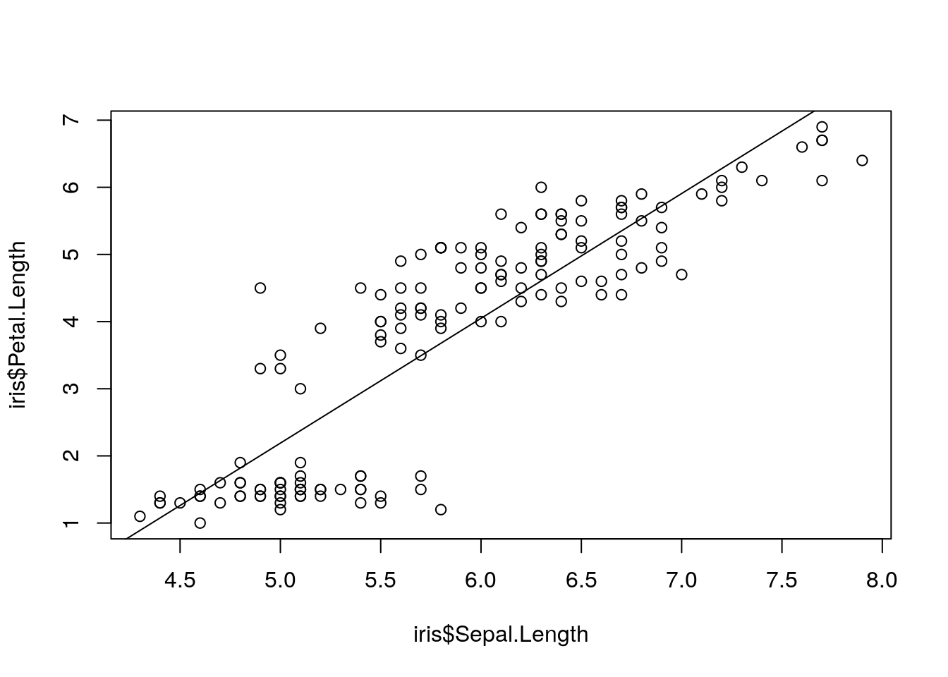
Figure 2: Petal vs. sepal length.
Is this also true for each species separately?
> plot(iris$Sepal.Length, iris$Petal.Length, col = as.numeric(iris$Species))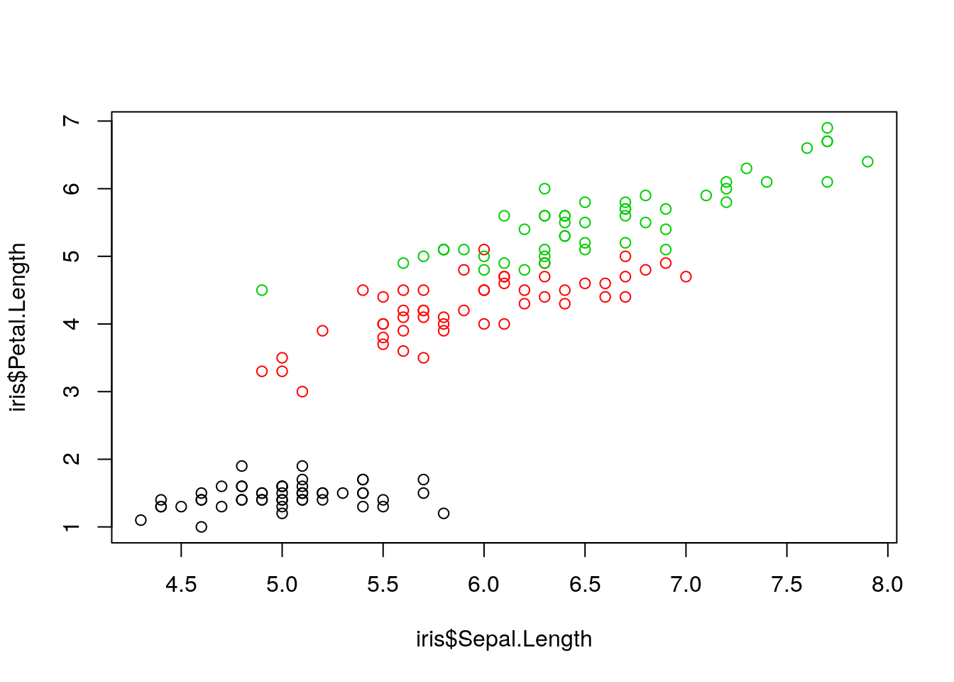
Figure 3: Petal vs. sepal length, by species.
> coplot(iris$Petal.Length ~ iris$Sepal.Length |
+     iris$Species, columns = 3)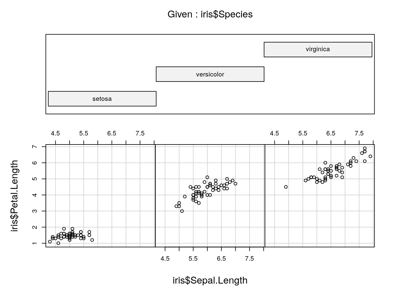
Figure 4: Petal vs. sepal length, using 'coplot'.
Mean comparison
Let's now look at the petal widths. Let's check if they vary by species:
> boxplot(iris$Petal.Width ~ iris$Species)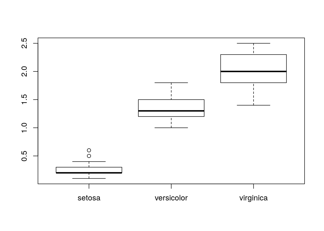
Figure 5: Petal width.
We're interested in comparing the means:
> mean(iris$Petal.Width[iris$Species == "setosa"])# [1] 0.246> by(iris$Petal.Width, iris$Species, mean)# iris$Species: setosa
# [1] 0.246
# -----------------------------------------------
# iris$Species: versicolor
# [1] 1.326
# -----------------------------------------------
# iris$Species: virginica
# [1] 2.026Based on their values only, these means seem clearly different. We can test them 2 by 2 with t tests (the parameter var.equal = TRUE indicates that the variances are equal within each group):
> t.test(iris$Petal.Width[1:50], iris$Petal.Width[51:100],
+     var.equal = TRUE)
#
# Two Sample t-test
#
# data: iris$Petal.Width[1:50] and iris$Petal.Width[51:100]
# t = -34.08, df = 98, p-value < 2.2e-16
# alternative hypothesis: true difference in means is not equal to 0
# 95 percent confidence interval:
# -1.142887 -1.017113
# sample estimates:
# mean of x mean of y
# 0.246 1.326> t.test(iris$Petal.Width[51:100], iris$Petal.Width[101:150],
+ var.equal = TRUE)#
# Two Sample t-test
#
# data: iris$Petal.Width[51:100] and iris$Petal.Width[101:150]
# t = -14.625, df = 98, p-value < 2.2e-16
# alternative hypothesis: true difference in means is not equal to 0
# 95 percent confidence interval:
# -0.7949807 -0.6050193
# sample estimates:
# mean of x mean of y
# 1.326 2.026> t.test(iris$Petal.Width[1:50], iris$Petal.Width[101:150],
+ var.equal = TRUE)#
# Two Sample t-test
#
# data: iris$Petal.Width[1:50] and iris$Petal.Width[101:150]
# t = -42.786, df = 98, p-value < 2.2e-16
# alternative hypothesis: true difference in means is not equal to 0
# 95 percent confidence interval:
# -1.862559 -1.697441
# sample estimates:
# mean of x mean of y
# 0.246 2.026Even though the difference are significant, we are limited by the multiplication of tests (if we had 10 classes, we would have needed 45 tests!) which ends up in multiplicative risks of error. This is why we need to use an analysis of variance (ANOVA) that can deal with this problem in one single test.
Partitioning the variance
The total variance can be split in a treatment variance and an error variance. Let's have a look at the total variance first:
> (totvar <- 1/nrow(iris) * sum((iris$Petal.Width -
+     mean(iris$Petal.Width))^2))
# [1] 0.5771329Let's compare this result with the output of the function var:
> var(iris$Petal.Width)# [1] 0.5810063> totvar * nrow(iris)/(nrow(iris) - 1)# [1] 0.5810063According to the documentation of var, "the denominator \(n - 1\) is used which gives an unbiased estimator of the variance for i.i.d. [independent and identically distributed] observations." We can create a function to compute the variance with a \(n\) denominator instead of \(n - 1\):
> varN <- function(x) 1/length(x) * sum((x - mean(x))^2)
> varN(iris$Petal.Width)
# [1] 0.5771329We can now proceed with the partitioning of the variance:
> iris$Mean <- rep(by(iris$Petal.Width, iris$Species,
+     mean), each = 50)
> (treatvar <- 1/nrow(iris) * sum((iris$Mean - mean(iris$Petal.Width))^2))
# [1] 0.5360889> (errvar <- 1/nrow(iris) * sum((iris$Petal.Width -
+ iris$Mean)^2))# [1] 0.041044Let's check that the total variance is equal to the sum of the other two:
> treatvar + errvar# [1] 0.5771329There is a dedicated function for an analysis of variance: the function aov, which gives directly the different sums of squares:
> aov(iris$Petal.Width ~ iris$Species)# Call:
# aov(formula = iris$Petal.Width ~ iris$Species)
#
# Terms:
# iris$Species Residuals
# Sum of Squares 80.41333 6.15660
# Deg. of Freedom 2 147
#
# Residual standard error: 0.20465
# Estimated effects may be unbalancedWe can compute the treatment and error variances based on the sums of squares:
> 80.41333/150# [1] 0.5360889> 6.1566/150# [1] 0.041044Tests and conclusions
The contribution of the treatment variance in the total variance is given by \(\eta^2 = V_{Treatments} / V_{Total}\):
> treatvar/totvar# [1] 0.9288829The actual ANOVA test can be performed with the ANOVA function, based on the linear model that we want to try:
> anova(lm(iris$Petal.Width ~ iris$Species))# Analysis of Variance Table
#
# Response: iris$Petal.Width
# Df Sum Sq Mean Sq F value Pr(>F)
# iris$Species 2 80.413 40.207 960.01 < 2.2e-16 ***
# Residuals 147 6.157 0.042
# ---
# Signif. codes: 0 '***' 0.001 '**' 0.01 '*' 0.05 '.' 0.1 ' ' 1Conclusions?
R session information
Before terminating, we can have a look at the information of the session:
> sessionInfo()# R version 3.3.3 (2017-03-06)
# Platform: x86_64-pc-linux-gnu (64-bit)
# Running under: Debian GNU/Linux 9 (stretch)
#
# locale:
# [1] LC_CTYPE=en_US.UTF-8 LC_NUMERIC=C
# [3] LC_TIME=en_US.UTF-8 LC_COLLATE=en_US.UTF-8
# [5] LC_MONETARY=en_US.UTF-8 LC_MESSAGES=en_US.UTF-8
# [7] LC_PAPER=en_US.UTF-8 LC_NAME=C
# [9] LC_ADDRESS=C LC_TELEPHONE=C
# [11] LC_MEASUREMENT=en_US.UTF-8 LC_IDENTIFICATION=C
#
# attached base packages:
# [1] methods stats graphics grDevices utils datasets
# [7] base
#
# loaded via a namespace (and not attached):
# [1] Rcpp_1.0.3 bookdown_0.18 codetools_0.2-15
# [4] digest_0.6.25 formatR_1.7 magrittr_1.5
# [7] evaluate_0.14 blogdown_0.18 highr_0.8
# [10] rlang_0.4.5 stringi_1.4.6 rmarkdown_2.1
# [13] tools_3.3.3 stringr_1.4.0 xfun_0.12
# [16] yaml_2.2.1 htmltools_0.4.0 knitr_1.28This shows in particular the version of R and the platform in which it is running, as well as all packages loaded, together with their version (it is beyond the scope of this introduction to describe the difference between "attached" and "loaded" packages; from a user's perspective, they are essentially the same thing).
Available at: https://www.r-project.org↩
Available at: https://cran.r-project.org/doc/manuals/R-intro.pdf↩
Available at: https://www.rstudio.com/↩
All these functions can be used on any data type, but will only be demonstrated here on data frames. Feel free to explore with other data types!↩
The standard behavior is to do it interactively when the user terminates a session.↩