April 11, 2018
Some theory of habitat selection
What is habitat?
- Short answer:
"By the habitat… is meant the kind of situation in which the organism lives." (McDougall, 1927)
- A little bit more complex:
"Resources and conditions present in an area that produce occupancy—including survival and reproduction—by a given organism." (Hall et al., 1997)
→ Inherently multivariate!
Why do we study habitat?
Critical to characterize a species habitat and how it is used.
- Research (ecology, evolution)
- Management
- Conservation
A simple example

| Type | # Locs | % Locs | % Surface | Ratio |
|---|---|---|---|---|
| A | 50 | 52.1 | 58 | 0.90 |
| B | 17 | 17.7 | 23 | 0.77 |
| C | 7 | 7.3 | 11 | 0.66 |
| D | 5 | 5.2 | 5 | 1.04 |
| E | 17 | 17.7 | 3 | 5.9 |
Habitat selection
Aim of habitat selection is to highlight relationships between the distribution of locations and environmental features.

- Environment: A set of environmental variables → AVAILABILITY
- Locations: Individuals can be identified or not → USE
→ Habitat selection is statistically defined as a disproportionate usage of available habitat.
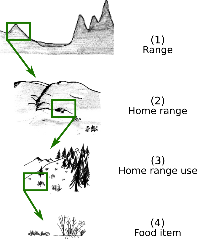
A hierarchical process (Johnson, 1980)
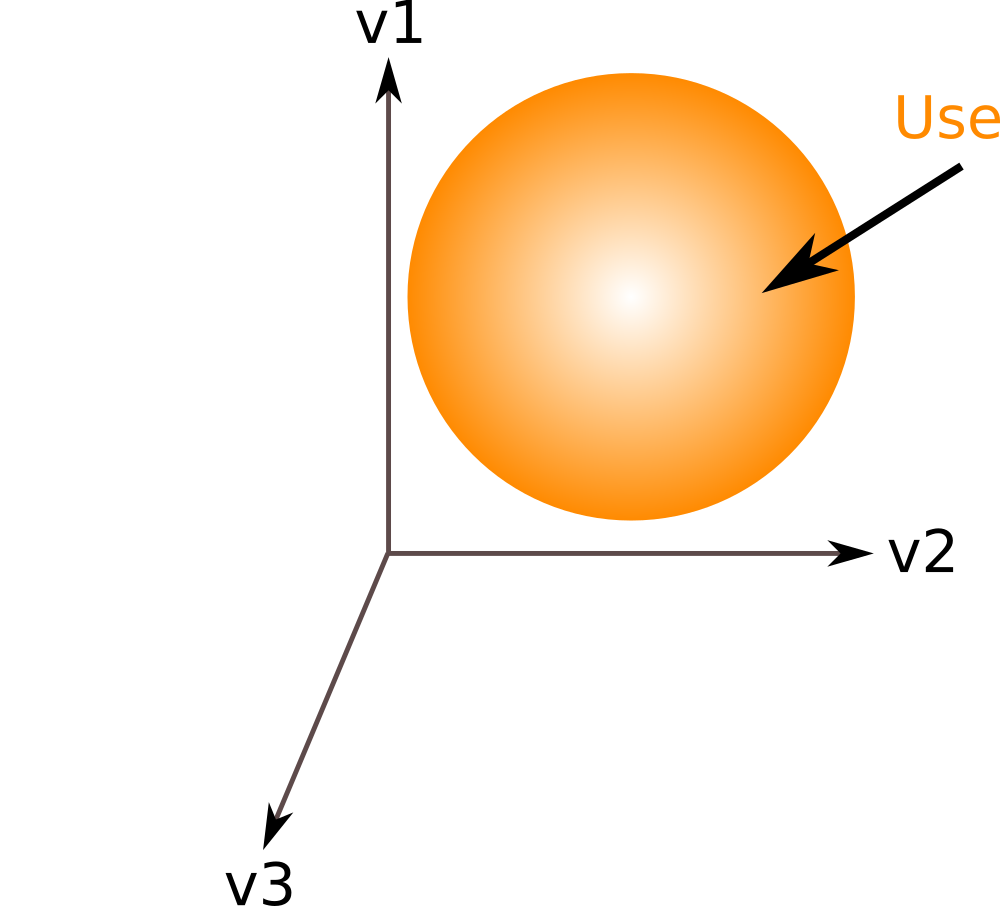
The geometric model of the Ecological Niche
Ecological niche
"An n-dimensional hypervolume, every point in which corresponds to a state of the environment which would permit the species to exist indefinitely"
- p environmental variables
- N locations in the ecological space
- (can be generalized to the individual)
Ecological niche
Ecological niche

In practice
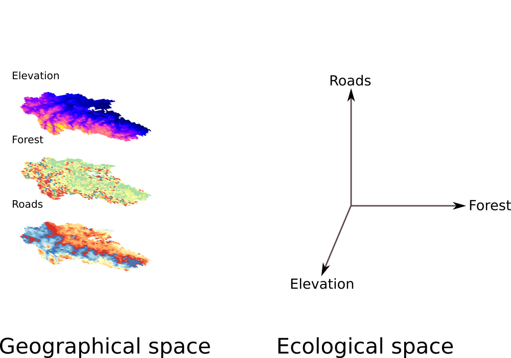
In practice

In practice
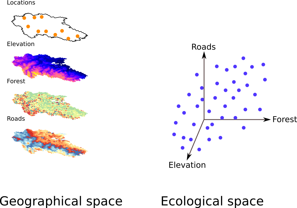
In practice

In practice

Niche analyses
- Exploration: multivariate analyses (PCA, ENFA, Mahalanobis distances, etc.)
- Modeling: regression analyses (RSF)
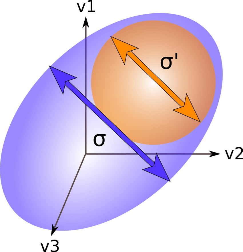
Marginality
- A difference of means: \(\mu - \mu\prime\)

Specialization (inverse of tolerance)
- A ratio of variance: \(\frac{\sigma}{\sigma\prime}\)
Study case
Locations and environmental data
The data come from the PhD of Daniel Maillard on wild boars (Sus scrofa) in Puéchabon (France). Six wild boards have been captured and monitored with radio-telemetry in July and August in the years 1993–1995.
During the day, wild boars rest in shelters, which have been located almost daily. We are trying to assess what are the habitat characteristics that wild boars look for to find shelter.
Maillard D. (1996) Occupation et utilisation de la garrigue et du vignoble méditerranéens par le sanglier (Sus scrofa L.). In: Biologie des populations et des écosystemes, 235 pp. Université de droit, d'économie et des sciences d'Aix-Marseille III.
Getting ready
Install necessary packages:
install.packages(c("adehabitatHS", "rgdal"))
Download and extract data.zip in your working directory, and download the R code 1.R:
download.file(
    "https://mablab.org/project/r/2018-04-11-niche-analyses/data.zip",
    "data.zip")
unzip("data.zip", exdir = "data")
file.remove("data.zip")
download.file(
    "https://mablab.org/project/r/2018-04-11-niche-analyses/1.R",
    "1.R")
Data import
library("adehabitatHS")
locs <- read.delim("data/locs.txt")
coordinates(locs) <- ~X+Y
head(locs)
##         coordinates   NOM
## 1 (699889, 3161560) Brock
## 2 (699291, 3161120) Brock
## 3 (700046, 3161540) Brock
## 4 (700050, 3161580) Brock
## 5 (699811, 3161390) Brock
## 6 (698840, 3161030) Brock
## Coordinate Reference System (CRS) arguments: NA
Data import
library("rgdal")
elev <- readGDAL("data/altitude.asc")
image(elev)
plot(locs, add = TRUE)

Data import
li <- lapply(list.files("data", pattern = ".asc",
    full.names = TRUE), readGDAL)
names(li) <- sub(".asc", "", list.files("data", pattern = ".asc"))
maps <- do.call(cbind, li)
fullgrid(maps) <- FALSE
names(maps) <- sub(".asc", "", list.files("data", pattern = ".asc"))
mimage(maps)

Habitat characterization: PCA
Structure in the environment
We check the presence of any structure with a Principal Component Analysis:
tab <- slot(maps, "data")
pc1 <- dudi.pca(tab)
s.corcircle(pc1$co)
maps$pc1 <- pc1$li[, 1]
maps$pc2 <- pc1$li[, 2]
mimage(maps)
Habitat selection at the population level: ENFA
Principle
- Population level: all individuals together (perfect for presence data)
- One axis of marginality
- Successive axes of specialization
- Pixels and variables are projected in the factorial plane just as for a PCA.
Application
pr <- slot(count.points(SpatialPoints(locs), maps), "data")[, 1]
enfa1 <- enfa(pc1, pr)
scatter(enfa1, pts = TRUE)
hist(enfa1)
hist(enfa1, scores = FALSE, type = "l")
maps$mar <- enfa1$li$Mar
mimage(maps)
Wrap-up
Working hypotheses
- Stable system (movement, population dynamic, resources)
- Available habitat correctly identified. Maybe the most complicated hypothesis… Must be defined by the biologist!
- Unbiased use data
- Free access to the entire habitat for all animals (selection is a choice)
- Resources affecting habitat selection correctly identified.
Other approaches
Several multivariate niche analyses:
- Population level: GNESFA (General niche-environment system factor analysis; Calenge & Basille, 2008), a generalization of the ENFA with several complementary methods (MADIFA, FANTER). Check the MADIFA to compute habitat suitability.
- Individual level: K-select (Calenge et al., 2005) and EISERA (Eigenanalysis of selection ratios; Calenge & Dufour, 2006) to investigate second- and third-order selection.
Warning!
Habitat selection is not simple:
- False absences: that the species is not detected does not mean the habitat is avoided!
- Detection problems
- Historical reasons
- Low use of some habitat does not mean it is useless (example: waterhole)
- Habitat selection, yes, but for what kind of activity? Foraging? Resting? Looking for mates?
References
- Basille, M.; Calenge, C.; Marboutin, É.; Andersen, R. & Gaillard, J.-M. (2008) Assessing habitat selection using multivariate statistics: Some refinements of the Ecological-Niche Factor Analysis. Ecological Modelling, 211:233–240.
- Calenge, C.; Dufour, A. & Maillard, D. (2005) K-select analysis: A new method to analyse habitat selection in radio-tracking studies. Ecological Modelling, 186: 143–153.
- Calenge, C. (2006) The package
adehabitatfor the R software: A tool for the analysis of space and habitat use by animals. Ecological Modelling, 197:516–519. - Calenge, C. & Dufour, A. B. (2006) Eigenanalysis of selection ratios from animal radio-tracking data. Ecology, 87:2349–2355.
- Calenge, C.; Darmon, G.; Basille, M.; Loison, A. & Jullien, J.-M. (2008) The factorial decomposition of the Mahalanobis distances in habitat selection studies. Ecology, 89:555–566.
- Calenge, C. & Basille, M. (2008) A general framework for the statistical exploration of the ecological niche. Journal of Theoretical Biology, 252:674–685.
References (continued)
- Hall, L. S.; Krausman, P. R. & Morrison, M. L. (1997) The habitat concept and a plea for standard terminology. Wildlife Society Bulletin, 25:173–182.
- Hirzel, A. H.; Hausser, J.; Chessel, D. & Perrin, N. (2002) Ecological-Niche Factor Analysis: How to compute habitat-suitability maps without absence data? Ecology, 83:2027–2036.
- Hutchinson, G. E. (1957) Concluding remarks. Cold Spring Harbour Symposium on Quantitative Biology, 22:415–427.
- Johnson, D. H. (1980) The comparison of usage and availability measurements for evaluating resource preference. Ecology, 61:65–71.
- McDougall, W. B. (1927) Plant ecology. Lee & Febiger.